Exponential Smoothing
Exponential Smoothing. Part 1 – Simple SES. Simple Exponential Smoothing (SES). Simple Exponential Smoothing.

Exponential Smoothing
E N D
Presentation Transcript
Exponential Smoothing Part 1 – Simple SES
Simple Exponential Smoothing • Random walk and average forecasts are the polar cases. We often want something in between – more than the most recent data is considered, but past data is weighted less heavily than recent data. • Simple exponential smoothing (SES) uses a weighted moving average with weights that decrease exponentially.
SES One-Step-Ahead Forecasting • In this case, 0 ≤ α ≤ 1 is a smoothing parameter. • The closer α is to 1, the less heavily past observations are weighted. If α = 1 you have the random walk (naïve) forecast.
Exponentially Weighted Average • The process has to start somewhere, so we let the first forecast of y1 be denoted by l0. Then:
Initialization • The last term in the weighted moving average is (1-α)Tl0 • So the value of l0 plays a role in all subsequent forecasts. • For sufficiently large T, the weight on this term is usually small. An exception would be if α is close to zero. • It is common to assign l0=y1, but a better alternative is to treat it as a parameter along with α.
Optimization • We can choose α and l0 by minimizing MSE: • Unlike regression there is no closed form solution – we need to use numerical optimization.
Simple Exponential Smoothing • A “flat” forecast function. Remember that a forecast is an estimated mean of a future value. • With no trend, no seasonality, and no other patterns, the forecasts are constant.
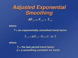
Next Step • Holt’s Local Trend Method: Holt (1957) extended SES to allow forecasting of data with trends. • After that, a minor modification to Holt allows exponential trends. • Then, trends with a damping parameter to make long-range forecasts more conservative.


