Download
1 / 24
250 likes | 430 Views
This chapter discusses curve fitting approaches such as least-squares regression and interpolation. It covers statistical concepts like normal distribution and linear regression methods for fitting straight lines. Examples and implementation techniques using MATLAB are also provided to better understand these methods.

E N D
Chapter 12Curve Fitting : Fitting a Straight LineGab-Byung Chae
Curve Fitting • Finding a function passing thru -May require estimates at points between the discrete values. -May require a simplified version of a complicated function.
12.1 Two general approaches for curving fitting • Least-squares regression • The data exhibits “scatter” • Interpolation • Where the data is known to be very precise, the basic approach is to fit a curve or a series of curves that pass directly through each of the points.
12.2 Statistics Review n data points y1,y2,…,yn mean standard deviation variance coefficient of variation degrees of freedom
The Normal Distribution • As n increases, the histogram often approaches the normal distribution. 68% of total measurements in
12.3 Least Squares Regression • Minimize some measure of the difference between the approximating function and the given data points. • In least squares method, the error is measured as :
Linear Least Squares Regression • f(x) is in a linear form : f(x)=ax+b • The error : e = y – ax - b • The sum of the residuals errors for all the variable data, as in • Does it work? -Any straight line passing through the midpoint of the connecting line get the minimum value • Then NO !
Is minimized when : -The minimum of E occurs when the partial derivatives of E with respect to each of the variables are 0. Equ. (12.15) and (12.16)
Example 12.2 • Find a function of a straight line that fits (10, 25), (20, 70), (30, 380), (40, 550), (50, 610), (60, 1220), (70, 830), (80, 1450) in least squares method.
The spread of the points around the line is of similar magnitude along the entire range of the data. • The distribution of these points about the line is normal. the estimates of a and b are the best!! This is called the maximum likelihood principle in statistics.
Standard Error of Estimate It is divided by n-2 since we lost two data a and b. Quantifies the spread around the regression line. Quantifies the spread around the mean.
Coefficient of Determination • correlation coefficient • r=1 => the line explains 100% of the variability of the data • r=0 => the fit represents no improvement over mean
Example 12.3 These results indicate that 88.05% of the original uncertainty has been explained by the linear model.
12.3.4 Linearization of Nonlinear Relationships The exponential equation The power equation The sturation-growth-rate equation
Example 12.4 • (10, 25), (20, 70), (30, 380), (40, 550), (50, 610), (60, 1220), (70, 830), (80, 1450) using power equation. (That is we assume we fit a power equation to the given data.) f(x) is in a linear form : f(x)=ax+b
MATLAB’s methods • z=polyfit(x,y,n) : n : the degree of the polynomial • yy=polyval(z,xx)