Curve-Fitting Polynomial Interpolation
Curve-Fitting Polynomial Interpolation. Curve Fitting. Regression Linear Regression Polynomial Regression Multiple Linear Regression Non-linear Regression Interpolation Newton's Divided-Difference Interpolation Lagrange Interpolating Polynomials Spline Interpolation.

Curve-Fitting Polynomial Interpolation
E N D
Presentation Transcript
Curve Fitting Regression Linear Regression Polynomial Regression Multiple Linear Regression Non-linear Regression Interpolation Newton's Divided-Difference Interpolation Lagrange Interpolating Polynomials Spline Interpolation
Interpolation • Given a sequence of n unique points, (xi, yi) • Want to construct a function f(x) that passes through all the given points so that … • We can use f(x) to estimate the value of y for any xinside the range of the known base points
Extrapolation • Extrapolation is the process of estimating a value of f(x) that lies outside the range of the known base points. • Extreme care should be exercised where one must extrapolate.
Polynomial Interpolation Objective: Given n+1 points, we want to find the polynomial of order n that passes through all the points.
Polynomial Interpolation • The nth-order polynomial that passes through n+1 points is unique, but it can be written in different mathematical formats: • The conventional form • The Newton Form • The Lagrange Form • Useful characteristics of polynomials • Infinitely differentiable • Can be easily integrated • Easy to evaluate
Characteristics of Polynomials • Polynomials of order n • Has at most n-1 turning points (local optima) • Hast at most n real roots • At most n different x's that makespn(x) = 0 • pn(x) passes through x-axis at most n times. • Linear combination of polynomials of order ≤ n results in a polynomial of order ≤ n. • We can express a polynomial as sum of polynomials.
Conventional Form Polynomial • To calculate a0, a1, …, an • Need n+1 points, (x0, f(x0)), (x1, f(x1)), …, (xn, f(xn)) • Create n+1 equations which can be solved for the n+1 unknowns as:
Conventional Form Polynomial • What is the shortcoming of finding the polynomial using this method? • This system is typically ill-conditioned. • The resulting coefficients can be highly inaccurate when n is large.
Alternative Approaches • If our objective is to determine the intermediate values between points, we can construct and represent the polynomials in different forms. • Newton Form • Lagrange Form
Constructing Polynomial • Let pn(x) be an nth-order polynomial that passes through the first n+1 points. • Given 3 points • We can construct p0(x) as p0(x) = f(x0) = 4 i.e., the 0th-order polynomial that passes through the 1st point.
Constructing Polynomial –p1(x) • We can construct p1(x) as p1(x) = p0(x) + b1(x – 1) for some constant b1 • At x = x0 = 1,b1(x – 1) is 0. Thus p1(1) = p0(1). • This shows that p1(x) also passes through the 1st point. • We only need to find b1 such that p1(x1) = f(x1) = 2. • At x = x1 = 2, p1(2) = p0(2) + b1(2– 1) => b1= (2 – 4) / (2 – 1) = -2 • Thus p1(x) = 4 + (-2)(x – 1)
Constructing Polynomial –p2(x) • We can construct p2(x) as p2(x) = p1(x) + b2(x – 1)(x – 2) for some constant b2 • At x = x0 = 1 andx = x1 = 2,p2(x) = p1(x). • So p2(x) also passes through the first two points. • We only need to find b2 such that p2(x2) = f(x2) = 5. • At x = x2 = 3, p1(3) = 4 + (-2)(3– 1) = 0 p2(3) = p1(3) + b2(3– 1)(3 – 2) => b2= (5 – 0) / 2 = 2.5 • Thus p2(x) = 4 + (-2)(x – 1) + 2.5(x – 1)(x – 2)
Constructing Polynomial –pn(x) • In general, given n+1 points (x0, f(x0)), (x1, f(x1)), …, (xn, f(xn)) • If we know pn-1(x) that interpolates the first n points, we can construct pn(x) as pn(x) = pn-1(x) + bn(x – x0)(x – x1)…(x – xn-1) where bn can be calculated as
Constructing Polynomial –pn(x) We can also expand pn(x) = pn-1(x) + bn(x – x0)(x – x1)…(x – xn-1) recursively and rewrite pn(x) as pn(x) = b0 + b1(x – x0) + b2(x – x0)(x – x1) + … + bn(x – x0)(x – x1)…(x – xn-1) where bi can be calculated incrementally as
Calculating the Coefficients b0, b1, b2, …, bn • A more efficient way to calculate b0, b1, b2, …, bn is by calculating them as finite divided difference b1: Finite divided difference for f of order 1 [f'(x) ] b2: Finite divided difference for f of order 2 [f"(x)]
Finite Divided Differences Recursive Property of Divided Differences • The divided difference obey the formula Invariance Theorem • The divided difference f[xk, …, x1, x0] is invariant under all permutations of the arguments x0, x1, …, xk.
Graphical depiction of the recursive nature of finite divided differences.
Example Construct a 4th order polynomial in Newton form that passes through the following points: We can construct the polynomial as
Example To calculate b0, b1, b2, b3, we can construct a divided difference table as
Example (Exercise) Calculate f[x1, x0] and f[x4, x3].
Example To calculate b0, b1, b2, b3, we can construct a divided difference table as
Example To calculate b0, b1, b2, b3, we can construct a divided difference table as
Example To calculate b0, b1, b2, b3, we can construct a divided difference table as
Example To calculate b0, b1, b2, b3, we can construct a divided difference table as
Example To calculate b0, b1, b2, b3, we can construct a divided difference table as b0 b1 b2 b3 b4 Thus we can write the polynomial as
Polynomial in Nested Newton Form • Polynomials in Newton form can be reformulated in nested form for efficient evaluation. • For example, can be reformulated in nested form as
Lagrange Interpolating Polynomials Construct a polynomial in the form
Lagrange Interpolating Polynomials • For example,
Example Construct a 4th order polynomial in Lagrange form that passes through the following points: We can construct the polynomial as where Li(x) can be constructed separately as … (see next page)
Lagrange Form vs. Newton Form • Lagrange • Use to derive the Newton-Cotes formulas for use in numerical integration • Newton • Allows construction of higher order polynomial incrementally • Polynomial in nested Newton form is more efficient to evaluate • Allow error estimation when the polynomial is used to approximate a function
Summary • Polynomial interpolation for approximate complicated functions. (Data are exact) • How to construct Newton and Lagrange Polynomial. • How to calculate divided difference of order n when given n+1 data points.
Interpolation Error ** • If pn(x) interpolates f(x) at x0, …, xn, then the interpolation is • When using pn(x) to approximate f(x) in an interval, one should select n+1Chebyshev nodes/points (as oppose to equally spaced points) from the interval in order to minimize the interpolation error.

