Ch11 Curve Fitting
Ch11 Curve Fitting. Dr. Deshi Ye yedeshi@zju.edu.cn. Outline. The method of Least Squares Inferences based on the Least Squares Estimators Curvilinear Regression Multiple Regression. 11.1 The Method of Least Squares.


Ch11 Curve Fitting
E N D
Presentation Transcript
Ch11 Curve Fitting Dr. Deshi Ye yedeshi@zju.edu.cn
Outline • The method of Least Squares • Inferences based on the Least Squares Estimators • Curvilinear Regression • Multiple Regression
11.1 The Method of Least Squares • Study the case where a dependent variable is to be predicted in terms of a single independent variable. • The random variable Y depends on a random variable X. • Regressing curve of Y on x, the relationship between x and the mean of the corresponding distribution of Y.
Linear regression • Linear regression: for any x, the mean of the distribution of the Y’s is given by In general, Y will differ from this mean, and we denote this difference as follows is a random variable and we can also choose so that the mean of the distribution of this random is equal to zero.
Analysis as close as possible to zero.
Principle of least squares Choose a and b so that is minimum. The procedure of finding the equation of the line which best fits a given set of paired data, called the method of least squares. Some notations:
Least squares estimators Fitted (or estimated) regression line Residuals: observation – fitted value= The minimum value of the sum of squares is called the residual sum of squares or error sum of squares. We will show that
EX solution • Y = 14.8 X + 4.35
X-and-Y • X-axis Y-axis independent dependent predictor predicted carrier response input output
Example • You’re a marketing analyst for Hasbro Toys. You gather the following data: • Ad $Sales (Units)1 1 2 1 3 2 4 2 5 4 • What is the relationshipbetween sales & advertising?
Scattergram Sales vs. Advertising Sales Advertising
11.2 Inference based on the Least Squares Estimators • We assume that the regression is linear in x and, furthermore, that the n random variable Yi are independently normally distribution with the means • Statistical model for straight-line regression are independent normal distributed random variable having zero means and the common variance
Standard error of estimate • The i-th deviation and the estimate of is Estimate of can also be written as follows
Statistics for inferences: based on the assumption made concerning the distribution of the values of Y, the following theorem holds. Theorem. The statistics are values of random variables having the t distribution with n-2 degrees of freedom. Confidence intervals
Example • The following data pertain to number of computer jobs per day and the central processing unit (CPU) time required.
EX • 1) Obtain a least squares fit of a line to the observations on CPU time
Example • 2) Construct a 95% confidence interval for α The 95% confidence interval of α,
Example • 3) Test the null hypothesis against the alternative hypothesis at the 0.05 level of significance. Solution: the t statistic is given by Criterion: Decision: we cannot reject the null hypothesis
11.3 Curvilinear Regression • Regression curve is nonlinear. • Polynomial regression: Y on x is exponential, the mean of the distribution of values of Y is given by Take logarithms, we have Thus, we can estimate by the pairs of value
Polynomial regression • If there is no clear indication about the function form of the regression of Y on x, we assume it is polynomial regression
Polynomial Fitting • Really just a generalization of the previous case • Exact solution • Just big matrices
11.4 Multiple Regression The mean of Y on x is given by Minimize We can solve it when r=2 by the following equations
Example • P365.
Multiple Linear Fitting X1(x), . . .,XM(x) are arbitrary fixed functions of x (can be nonlinear), called the basis functions normal equations of the least squares problem Can be put in matrix form and solved
Correlation Models • 1. How strong is the linear relationship between 2 variables? • 2. Coefficient of correlation used • Population correlation coefficient denoted • Values range from -1 to +1
Correlation • Standardized observation • The sample correlation coefficient r
Coefficient of Correlation Values No Correlation -1.0 -.5 0 +.5 +1.0 Increasing degree of negative correlation Increasing degree of positive correlation