Download
1 / 27
270 likes | 290 Views
Explore the latest developments in improving TITAN nowcasting techniques by enhancing echo tracking methodologies. Learn about separating convective regions from stratiform areas and applying spatial scaling to improve forecast lead time. Discover how to correct tracking errors using Optical Flow and examples of convective outbreaks and storm identification improvements. Enhance your storm tracking skills with advanced methodologies.

E N D
Developments in echo tracking - enhancing TITAN Nowcasting Techniques 7.6 ERAD 2014 2 September 2014 Mike Dixon1 and Alan Seed2 1National Center for Atmospheric Research, Boulder, Colorado 2Centre for Australian Weather and Climate Research, Melbourne, Australia
Current work on TITAN enhancements Separating convective regions from stratiform areas prior to storm identification Applying spatial scaling to storm objects appropriately for forecast lead time Correcting tracking errors using Optical Flow
Handling mixed convective / stratiform situations(a) Identify the convective regions within the radar volume(b) Constrain the storm identification to the convective regions only
Example of scene with large regions of stratiform / bright-band,along with embedded convection Vertical section along line 1-2 Convectivearea Stratiformarea Column-max reflectivity Convection Bright-band
TITAN tends to merge both the convective and stratiform regionsinto a single storm identification.Therefore we need to isolate the convective regions. Merged convective andstratiform regions
The Steiner et. al (1995) method for convective partitioning was tested.However, it seemed to over-identify convective areas. The Steiner method computes the difference betweenthe reflectivity at a point and the ‘background’ reflectivity defined as the mean within 11 km of that point. The method identifies the convective regions based on the reflectivity difference, determining the radius of convective influence as a function of the background value. Stratiformarea
A modified method was developed, based on the ‘texture’ of reflectivity surrounding a grid point. ‘Mean texture’ of reflectivity – mean over the column oftexture = sqrt(sdev(dbz2))computed over a circular kernel 5km in radius,for each CAPPI height. Convective (cyan) vs Stratiform (blue)partition computed by thresholdingtexture at 15 dBZ
Storm identification on all regionscompared with using the convective regions only Storms identified using a 35 dBZ threshold. The storms include the regions of bright-band,leading to erroneously large storm areas Storms using the same 35 dBZ threshold but including only the convective regions
Example of convective partitioning for single radar with extensive bright-band 1 degree PPI for radar near Sydney Australia.Extensive stratiform region to the NE of the radar. Vertical section (1-2) showing bright-band near the radar and convection further away Stratiformregion Bright-band
Computing the texture and creating the partition for the single-radar case Mean reflectivity texture over all levels Convective areas shown in gray,with TITAN storm tracks
TITAN storms for all areas (left)and convective areas only (right) TITAN storms including stratiform areas TITAN storms on convective areas only
Spatial scaling appropriate for longer-term nowcasts - investigating approaches for a 2-hour lead time. For nowcasts of 30 to 60 minutes, the scale of storms as measured by the radars is appropriate. For longer lead time forecasts, say 1 hour to 2 hours, we want to identify and track only larger scale features, so we need a technique to isolate those features.
From Seed (2003) event lifetime vs. spatial scalebased on computed median correlation time for precipitation events 2 hrs 30 mins ~12km ~50km A. Seed, J Appl Meteor, Vol 42, No 3, March 2003.
From Germann et. al (2006), for an expected lifetime of 2 hours,the spatial scale should be between 32 and 64 km.We choose to test with a spatial scale of 50 km. 2 hr lifetime~50 kmspatial scale 30 min lifetime~8 kmspatial scale Germann et. al, J Atmos, Vol 63, No 8, August 2006.
Computing the spectrum of the reflectivity field shows the spatial frequency of the scene Reflectivity over a 1200km x 1200 km grid 2D FFT-based spectrum of reflectivity field
Computing the spectrum of the reflectivity field shows the spatial frequency of the phenomenon Reflectivity filtered for features 50 km and larger Spectrum filtered to retain features of 50 km scale and larger This includes the stratiform regions. What if we use this procedure on the convective areas only?
Applying the 50km spatial filter to the convective regions highlights the larger scale convective features Convective reflectivity regions Convective reflectivity filtered for features 50 km and larger
Comparing convective storm identificationat different scales Identification of smaller-scale convective features, minimum size 30 km2 Identification of features at the 50km spatial scale, minimum size 2500 km2
How well did we do with forecasting the linefiltered using a 50 km spatial filter? Forecast at 23:05 UTC on 2014/06/08. Shown are4 x 30 minute forecasts, to 2 hours. 2-hour verification at 01:05 UTC on 2014/06/09.This demonstrates that we can have some success forecasting large-scale features at longer lead times.
Sometimes we get tracking errors in challenging situations Example of radar scanning at 10 minute intervals, with fast moving storms.This can lead to problems with correct tracking.
Using a field tracked such as Optical Flow allows us toestimate the ‘background’ movement of the echoes.
Example of tracking errors.Neither storm in the NE quadrant is correctly tracked. In this case no overlap occurs because of small storm sizes, long time between scans and fast movement.
By applying the Optical Flow vectors to storms with short histories,we can improve both tracking the forecast accuracy.
Using TITAN, you can have some fun and animate the event as it unfolds Thank you