Download
1 / 24
240 likes | 423 Views
Literature Discussion, Zeuthen, October 18th 2004. The Unified Approach to the Classical Statistical Analysis of Small Signals (Feldman-Cousins). Ullrich Schwanke Humboldt University Berlin. Overview. Reminder: Some basic statistics Problems with classical confidence intervals

E N D
Literature Discussion, Zeuthen, October 18th 2004 The Unified Approach to the Classical Statistical Analysis of Small Signals(Feldman-Cousins) Ullrich Schwanke Humboldt University Berlin
Overview • Reminder: Some basic statistics • Problems with classical confidence intervals • The Unified Approach of Feldman & Cousins • Example: Gaussian PDF • Example: Poissonian process with background • Advanced Problems • Upper limits for fewer events than expected • systematic errors Paper I Paper II (and others) Paper I: Feldman and Cousins, Phys. Rev. D 57, 3873 (1998) Paper II: Hill, Phys. Rev. D 67, 118101 (2003)
Confidence Intervals confidence interval (CL=68.3%) x rate or flux or # of events confidence interval (CL=99%) • (Frequentist) Definition of the confidence interval for the measurement of a quantity x: • If the experiment were repeated and in each attempt a confidence interval is calculated, then a fraction of the confidence intervals will contain the true value of x (called ). A fraction 1- of the confidence intervals will not contain . • Note: Experiments must not be identical
Coverage • Confidence intervals overcover (i.e. are too conservative) • Reduced power to reject wrong hypotheses • Confidence intervals undercover • Measurement pretends to be more accurate than it actually is • Correct coverage Proper coverage can be tested by Monte Carlo simulations
Flip-Flopping The flip-flopping attitude (example): „We will state a measurement with a 1 error (i.e. CL=68.3%) if the measurement result is above m, and an 99% CL upper limit otherwise.“ • Flip-flopping between measurements and upper limits with different confidence levels spoils the coverage of the stated confidence intervals • Easy to show with a toy Monte Carlo
Flip-Flopping (II) • MC Simulation, measured value x from from G(,1), i.e. =1 • Calculated upper limit for x<3, assumed proper coverage there • Calculated confidence interval for x>3: x±1 • Undercoverage around 2, overcoverage for 4 Coverage (%) Fraction of central confidence intervals True mean Coverage is spoilt by deciding between central confidence interval (measurement) and limit based on data.
Feldman & Cousins Approach • Provides confidence intervals that change smoothly from upper limits to measurements • „User“ just needs to decide for a confidence level • Flip-flopping problem is solved • Uses Neyman‘s construction and a Likelihood Ratio to decide what values are included into confidence intervals
Neyman‘s Construction True value Measured value PDF e.g.
Neyman‘s Construction True value Measured value PDF e.g.
=5.0 =0.5 =0.1 F&C: Likelihood Ratio fixed „best“, physically allowed • Likelihood Ratio determines what x‘s are included into the confidence interval for a given
Measurement with symmetric errors, e.g. 6.0 1.6 • Confidence interval is 0..UL, i.e. upper limit • Measurement with asymmetric errors, e.g. F&C Confidence Intervals CL=90%
F&C: Coverage • (Pure) Feldman Cousins provides proper coverage
Poissonian Distribution • Poissonian process (true rate ) with background b • Measurement is number of events n, predicted background b (here assumed to be known without error) • n discrete confidence level can only be reached approximately slight (conventional) overcoverage • Likelihood Ratio:
Poissonian Distribution (II) • Note: upper limit for n=0 is 1
Intermediate Summary • Feldman Cousins solves flip-flopping problem • Everything 100% frequentist up to now • Poisson case: limit for n=0 seems low • How to include systematic uncertainties of signal and background efficiency into confidence interals? We are done with Paper I !
The KARMEN Anomaly • Check LSND result on Neutrino oscillations • No events detected, expected 2.9 background events • F&C upper limit is 1.1 for b=2.9 • But: F&C upper limit is 2.44 for b=0 • A worse experiment yields a better limit! • Background prediction should not affect upper limit if no events are seen!
The KARMEN Anomaly - Solutions • Replace „0“ by 1, 2, or Bayesian expectation value in • Apply conditioning (i.e. use a PDF that reflects the fact that the number of background events cannot exceed the number of actually measured events)
The KARMEN Anomaly - Solutions • Woodroofe & Roe, Phys. Rev. D 60, 053009 (1999) • „Some“ problems with proper coverage since PDF depends on measured n • Slight overcoverage
Inclusion of Systematic Errors • Inclusion of systematic errors usually involves Bayesian elements (ensemble of systematic errors) • (Frequentist) coverage not ensured, (approximate) Bayesian coverage • Example: interpret background expectation as Gaussian bb • Add (relative) systematic error on signal efficiency: Cousins & Highland, NIM A 320, 331 (1992)
Likelihood Ratio • PDF: background known without error, syst. error on signal efficiency is integrated out Poissonian Gaussian • Construct confidence intervals (in a 1D) for signal expectation s=s, Likelihood Ratio (a la F&C): Conrad et al., Phys. Rev. D 67, 012002 (2003)
Modified Likelihood Ratio • The standard Likelihood Ratio was found to give upper limits that decrease when systematic uncertainties are increased • Replace by • Widening effect of shifted acceptance intervals to higher n lower upper limits • Approach yields limits that behave as expected Paper II
Systematic Errors: Gaussian PDF • Example: Gaussian PDF with boundary condition () PDF s= 0 % s=10 % s=20 % s=30 % s=5 % Measured x for =3 True mean • Example: Gaussian PDF (=1) with boundary condition () and a systematic error on x of s % • H.E.S.S.: x corresponds to flux, s=15-20%
Systematic Errors: Gaussian PDF • Systematic error widens confidence belt (as expected) • Effect small for small since systematic error is relative CL=90% CL=90% + 20% syst. error AMANDA/IceCube: Poissonian PDF and dedicated codes for calculation of confidence intervals
Discussion Thanks