Download
1 / 17
180 likes | 343 Views
Explore classical statistical mechanics in the canonical ensemble, focusing on the classical ideal gas. Learn about phase space, Hamiltonian formulation, canonical distribution, partition function, thermodynamic averages, free energy, entropy, and classical ideal gas properties.

E N D
Classical Statistical Mechanicsin the Canonical Ensemble: Application to the Classical Ideal Gas
Canonical Ensemble in ClassicalStatistical Mechanics As we’ve seen, classical phase space for a system with f degrees of freedom is f generalized coordinates & f generalized momenta (qi,pi). The classical mechanics problem is done in the Hamiltonian formulation with a Hamiltonian energy function H(q,p). There may also be a few constants of motion (conserved quantities): energy, particle number, volume, ...
The Canonical Distribution in Classical Statistical Mechanics • The Partition Functionhas the form: • Z ≡ ∫∫∫d3r1d3r2…d3rN d3p1d3p2…d3pN e(-E/kT) • A 6N Dimensional Integral! • This assumes that we’ve already solved the classicalmechanics problemfor each particle in the system so that we know the total energy E for the N particles as a function of all positions ri& momentapi. • E E(r1,r2,r3,…rN,p1,p2,p3,…pN)
CLASSICAL Statistical Mechanics: • Let A ≡any measurable, macroscopic quantity. The thermodynamic average of A ≡<A>. This is what is measured. Use probability theory to calculate <A> : P(E) ≡ e[- E/(kBT)]/Z <A>≡ ∫∫∫(A)d3r1d3r2…d3rN d3p1d3p2…d3pNP(E) Another 6N Dimensional Integral!
Relationship of Z to Macroscopic Parameters Summary of the Canonical Ensemble (Derivations are in the book! Results are general & apply whether it’s a classical or a quantum system!) Mean Energy: Ē E = -∂(lnZ)/∂β <(ΔE)2> = [∂2(lnZ)/∂β2] β = 1/(kBT),kB =Boltzmann’s constant. Entropy: S = kBβĒ+ kBlnZ An important, frequently used result!
Summary of the Canonical Ensemble: Helmholtz Free Energy: F = E – TS = – (kBT)lnZ Note that this gives: Z = exp[-F/(kBT)] dF = S dT – PdV, so S = – (∂F/∂T)V, P = – (∂F/∂V)T Gibbs Free Energy: G = F + PV = PV – kBTlnZ. Enthalpy: H = E + PV = PV – ∂(lnZ)/∂β
Summary of the Canonical Ensemble: Mean Energy: Ē = – ∂(lnZ)/∂ = - (1/Z)(∂Z/∂) Mean Squared Energy: <E2> = (rprEr2)/(rpr) = (1/Z)(∂2Z/∂2) nth Moment: <En> = (rprErn)/(rpr) = (-1)n(1/Z)(∂nZ/∂n) Mean Square Deviation: <(ΔE)2> = <E2> - (Ē)2 = ∂2lnZ/∂2 = -∂Ē/∂. Constant Volume Heat Capacity CV = (∂Ē/∂T)V = (∂Ē/∂)(d/dT) = - kBT2(∂Ē/∂)
The Classical Ideal Gas • So, in Classical Statistical Mechanics, the • Canonical Probability Distribution is: • P(E) = [e-E/(kT)]/Z • Z ≡ ∫∫∫d3r1d3r2…d3rN d3p1d3p2…d3pN e(-E/kT) • This is the tool we will use in what follows. • As we.ve seen, from the partition function • Z all thermodynamic properties can be • calculated: pressure, energy, entropy….
Consider an Ideal Gas from the point of • view of microscopic physics. It is the • simplest macroscopic system. • Therefore, its useful use it to introduce the • use of the • Canonical Ensemble in Classical • Statistical Mechanics. • The ideal gas Equation of State is • PV= nRT • n is the number of moles of gas.
We’ll do Classical Statistical • Mechanics, but very briefly, lets • consider the simple Quantum • Mechanicsof an ideal gas & the take • the classical limit. • From the microscopic perspective, an • ideal gas is a system of Nnon • Interacting particles of mass m in a • volume V = abc. • (a, b, c are the box’s sides)
Since there is no interaction, each • molecule can be considered a “Particle • in a Box” as in elementary quantum • mechanics. • The energy levels for such a system • have the form: • where nx, ny, nx = integers
The energy levels for each molecule in the • Ideal Gas are: • l • (nx, ny, nx = integers) • (1) • The Ideal Gas molecules are non • interacting, so the gas Partition Function • has the simple form: • Z = (q)N (2) • where q One Particle Partition Function
Ideal Gas Partition Function: • Z = (q)N (2) • q One Particle Partition Function • Using (2) in the • Canonical Ensemble • formalism gives the • expressions on the • right for: mean energy • E, equation of state P • & entropy S:
The Partition Function for the 1- • dimensional particle in a “box” • under the assumption that the • energy levels are so closely spaced • that the sum becomes an integral • over phase space can be written: (3)
(3) • For the 3 – dimensional particle in a • “box”, the 3 dimensions are • independent so that the Partition • Function can be written as the product • of 3 terms like equation (3). That is: (4)
Using the Canonical • Ensemble expressions • from before: • The Mean Energy & • the Equation of • State can be obtained • (per mole): • To obtain, for one mole of gas:
The Entropycan also be obtained: E (5) • As first discussed by Gibbs, the Entropy • in Eq. (5) is NOT CORRECT! • Specifically, its dependence on particle • number N is wrong! • “Gibbs’ Paradox” • in the first part of Ch. 7!