Download
1 / 23
230 likes | 258 Views
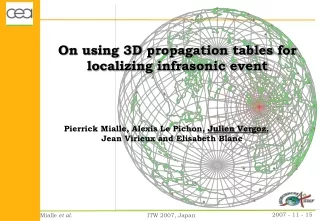
A presentation on the use of 3D propagation tables to localize infrasonic events, taking into account atmospheric variability. The presentation covers ray tracing with WASP 3D Sph, construction of propagation tables, and localization using bounce order tables. The variability of global propagation in space and time is also discussed.

E N D
On using 3D propagation tables for localizing infrasonic event Pierrick Mialle, Alexis Le Pichon, Julien Vergoz, Jean Virieux and Elisabeth Blanc
Problematic • Aim:localize infrasound events • On a global scale using sophisticated atmospheric specifications • Designed for operational purposes: reasonable computing time • Significant progress in the last years [Brown, 2002; Drob, 2003; O’Brien, 2004] • Account for moving medium in space and time: significant short time and range fluctuations • Tool • Source localization using global propagation tables centered on stations Propagation tables are carried out with WASP 3D Sph code
Outline of the presentation • Ray tracing with WASP 3d Sph • Ray tracing tool and atmospheric variability • Towards a WASP 3D Sph designed for propagation tables • Construction of the propagation tables • Regular tables • Advanced tables to reach the target • Localization using bounce order tables • Variability of global propagation in space and time
Variability of the medium along the trajectory 180 Atmospheric grid 140 Altitude (km) source 40 station 0 0.3 0.45 0.6 Effective sound speed (km/s) 160 120 Altitude (km) 80 40 0 Source 200 400 0 Station Distance (km) Ray tracing WASP-3D Sph & spatio-temporal variability of atmosphere WASP 3D Sph = Windy Atmospheric Sonic Propagation 3D in Spherical coordinates Ray tracing Propagation tables Regular Advanced Localization with bounce order Global variability Conclusion (3D paraxial ray theory-based method in spherical coordinates) Escaping rays Thermospheric [Virieux, 2004 & Dessa, 2005] Stratospheric Tropospheric Escaping rays (high thermosphere, above 120 km) It Is Iw
Regular propagation tables DR Dq Dh 3D mapping on large scale of infrasonic phases Ray tracing Propagation tables Regular Advanced Localization with bounce order Global variability Conclusion • Space and time dependent tables centred on a station • Every cell is associated with a source • 3D concentric source grid • 2D horizontally (radiusΔR and angle Δθ) with evolving steps (ΔR ~ RΔθ) • 1D vertically (height Δh) • Grid for atmospheric models fits the source mesh Integration box Mesh evolution ΔR ~ RΔθ • For each cell • Launchandcount rays reaching the integration box • Phase identification: Iw (<20km), Is (<70km) and It (>70km), statistics on phases and filling of the tables • Build propagation tables • Travel time, azimuth deviation, celerity, attenuation (atmospheric absorption [Sutherland and Bass, 2004] and/or geometrical spreading)
Regular propagation tables (cont.) Ray tracing Propagation tables Regular Advanced Localization with bounce order Global variability Conclusion Atmospheric data Station Concentric source grid Regular discretization of incidence & azimuth Ray tracing simulations with WASP 3D SPH For all stations detecting the event Propagation tables Localization
How to read propagation tables ? Ray tracing Propagation tables Regular Advanced Localization with bounce order Global variability Conclusion Is celerities Effective Stratospheric winds@ 40 km m/s m/s -130 m/s Flers +90 m/s Stratospheric jet • Strong stratospheric jet toward the south-east • Large variations of celerities Buncefield case Flers Station 2005-12-11 6:00 UT NRL-G2S
Thermospheric Tables Δθ (°) Celerity Stratospheric Tables Celerity Δθ (°) Ray tracing Propagation tables Regular Advanced Localization with bounce order Global variability Conclusion Flers Flers • Significant variations are observed: • Azimuth deviation: -15 to 15° • Celerity Is and It : 240-320 / 200-320 m/s • Local discontinuities of results Flers Flers Buncefield case Flers Station 2005-12-11 6:00 UT NRL-G2S
Local influences on global tables Buncefield case Flers Station 2005-12-11 6:00 UT NRL-G2S Altitude (km) Ray tracing Propagation tables Regular Advanced Localization with bounce order Global variability Conclusion Source thermospheric Phase conversions X-axis (km) tropospheric stratospheric Flers station • Regular table = uncomplete • For a given atmosphere specifications, how to distribute a finite number of rays to optimize the completion rate of the cells ? Advanced Tables Y-axis (km)
Advanced propagation tables Atmospheric data Station Ray tracing Propagation tables Regular Advanced Localization with bounce order Global variability Conclusion Concentric source grid Regular discretization of incidence & angles Ray tracing simulations with WASP 3D Sph Hunt for transition zones « Shooting Method »: reach the station For all stations detecting the event Propagation table Localization
Advanced tables Regular tables Celerity Celerity Celerity Ray tracing Propagation tables Regular Advanced Localization with bounce order Global variability Conclusion Thermospheric Regular vs Advanced • Surface completion rate is between 10 to 25% highers • Number of rays retrieved by cell is constrained (only closest rays to station) • More reliable and precise results • Computing cost is also larger (up to twice as much, ~10h for a grid radius of 3000km, 936 cells, and atmospheric perturbations) Celerity • Review of the phase mean celerities Stratospheric Flers Station 2005-12-11 6:00 UT NRL-G2S
3 6 1 2 4 5 Δθ (°) 4 6 3 1 2 5 15 10 5 0 0 -5 -10 Is6 Is7 Is8 Is9 Is10 Is5 -15 Is10 Is9 Is8 Is7 Is6 Is5 The Buncefield fire(BGS 2005-12-11 06:01:32 (UTC) 51.78° N / 0.43° W with ML2.2) • Tables by bounce order At I26DE Dq = 0.6° Dq = -1° Dq = -0.6° Dq = -0.5° Dq = 0.0° Dq = 0.1° 0.44 Is11 0.42 0.40 0.38 0.36 0.34 Is4 V (km/s)
3 6 2 4 5 1 C (m/s) 3 4 6 1 2 5 320 300 280 260 240 220 Is6 Is7 Is8 Is9 Is10 Is5 Is10 Is8 Is7 Is6 Is5 The Buncefield fire(BGS 2005-12-11 06:01:32 (UTC) 51.78° N / 0.43° W with ML2.2) • Tables by bounce order At I26DE Cel=270m/s Cel=320m/s Cel=300m/s Cel=290m/s Cel=285m/s Cel=280m/s 0.44 Is11 0.42 0.40 Is9 0.38 0.36 0.34 Is4 V (km/s)
Localization using tables by bounce order Localization with 6 predicted arrivals at I26DE, 2 at IGADE and 1 at Flers Ray tracing Propagation tables Regular Advanced Localization with bounce order Global variability Conclusion Localization errors with azimuth • With fastest phases and without correction: 52.6km • With fastest phases at 3 stations: 27.0km • With all predicted arrivals at 3 stations: 13.2km Localization errors with azimuths and travel times For I26DE and Flers, localization has been performed by minimizing a Misfit function (weighting both azimuth and travel time) [Sambridge and Gallagher, 1993] • Localization errors with the Misfit function: 6.5 km [Mialle, 2007]
Infrasonic propagation using tables Ray tracing Propagation tables Regular Advanced Localization with bounce order Global variability Conclusion Global scale variability • Tables for 7 IMS stations along a meridian • Seasonal variability • Spatial variability • Atmospheric model effects HWM / ECMWF
340 320 300 280 260 240 15 10 5 0 -5 -10 -15 60 55 50 45 40 35 30 Stratospheric tables with ECMWF for I02AR in 2003 October January April July (m/s) Ray tracing Propagation tables Regular Advanced Localization with bounce order Global variability Conclusion Celerity (°) Azimuth deviation (km) Turning height
Celerity ECMWF HWM Ray tracing Propagation tables Regular Advanced Localization with bounce order Global variability Conclusion • Almost all the surface is covered (less than 1.5% of empty cells) • Better covering of Is with ECMWF (+10 to 20%) and almost no Iw with HWM Surface (with respect to the total surface covered by the table) • Large spatial variations: steady close to the equator – perturbed around the tropics and higher • Significant model variations: for Is and Iw
Conclusion Ray tracing Propagation tables Regular Advanced Localization with bounce order Globalvariability Conclusion • Pre-localization: regular tables • With empiric atmospheric models (HWM/MSIS-E) roughly similar from one year to another • Storage of tables for each station over one year and for specific dates (seasonal & sub-seasonal effects) and time (diurnal effects) • Refined localization: advanced tables • More sophisticated available atmospheric models (ECMWF or NRL-G2S) • Reduced source grid centered on the pre-localization • What next? • Implementation and validation of the method in the French NDC operational system
Thank you for you attention ! ども ありがと
Regular discretization of ray parameters Ray parameters vs effective slowness Mean effective slowness + standard deviations 160 120 Altitude (km) 80 40 0 1.5 2.0 2.5 3.0 3.5 Effective slowness (km/s)
Optimized discretization of ray parameters Hunt for transitions Ray parameters vs effective slowness Mean effective slowness + standard deviations 160 120 Altitude (km) Escaping rays Detected transition zones 80 40 Iw-Is Is-It 0 1.5 2.0 2.5 3.0 3.5 Effective slowness (km/s)
Reach the target by a shooting method • 1st set of rays (with emission parameters i(1) and α(1)) distance • 2nd set of rays (with emission parameters i(2) and α(2)) Perturbations δiand δα distance • Final set of rays (i(3) and α(3)) obtained through quasi linearization Need for new i(3) and α(3) The goal is to reach the station Assuming One can then find the needed emission parameters
Is celerities m/s Source Flers Propagation direction