Download
1 / 16
170 likes | 426 Views
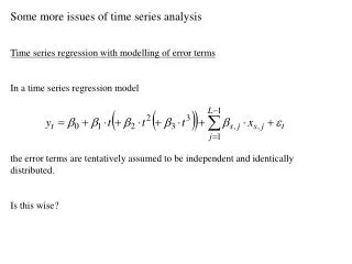
Some more issues of time series analysis Time series regression with modelling of error terms In a time series regression model the error terms are tentatively assumed to be independent and identically distributed. Is this wise?.

E N D
Some more issues of time series analysis Time series regression with modelling of error terms In a time series regression model the error terms are tentatively assumed to be independent and identically distributed. Is this wise?
Performing e.g. the Durbin-Watson test we may quite easily answer the question whether they are or not. • What if D-W gives evidence of serial correlation in the error terms? • Apply an AR(p) model to the error terms at the same time as the rest of the model is fitted. • Standard procedure: • Study the residuals from an ordinary regression fit • Identify which order p of the AR-model that may be the most appropriate for the error terms. • Make the fit of the combined regression-AR-model
Estimation can no longer be done using ordinary least-squares. Instead the conditional least-squares method is used. Procedures are not curretly available in Minitab, but in more comprehensive computer packages such as SAS and SPSS. Example Consider again the Hjälmaren month data set (that is used in assignments for weeks 36, 39 and 41)
Minitab output from an ordinary time series regression: The regression equation is Discharge.m = 83.1 - 0.0300 Time.m + 2.79 Jan + 6.36 Feb + 7.89 Mar + 16.1 Apr + 12.2 May - 5.06 Jun - 10.9 Jul - 10.1 Aug - 10.3 Sep - 10.1 Oct - 4.64 Nov Predictor Coef SE Coef T P Constant 83.13 33.60 2.47 0.013 Time.m -0.03000 0.01727 -1.74 0.083 Jan 2.795 2.613 1.07 0.285 Feb 6.359 2.613 2.43 0.015 Mar 7.887 2.613 3.02 0.003 Apr 16.145 2.613 6.18 0.000 May 12.228 2.613 4.68 0.000 Jun -5.059 2.613 -1.94 0.053 Jul -10.938 2.613 -4.19 0.000 Aug -10.144 2.613 -3.88 0.000 Sep -10.278 2.613 -3.93 0.000 Oct -10.138 2.613 -3.88 0.000 Nov -4.638 2.613 -1.77 0.076 S = 19.1121 R-Sq = 18.8% R-Sq(adj) = 18.1%
Residual plots Residuals seem to follow an AR-model with order 1 or 2
SPSS output of a regression analysis with error term modelled as AR(1) FINAL PARAMETERS: Number of residuals 1284 Standard error 15.210763 Log likelihood -5310.1953 AIC 10648.391 SBC 10720.599 Variables in the Model: B SEB T-RATIO APPROX. PROB. AR1 .605651 .022323 27.130704 .00000000 JAN 2.641382 1.644536 1.606156 .10848820 FEB 6.239922 2.077007 3.004285 .00271421 MAR 7.788472 2.295270 3.393270 .00071191 APR 16.059974 2.411374 6.660092 .00000000 MAY 12.151510 2.468703 4.922224 .00000097 JUN -5.129816 2.485909 -2.063557 .03926251 JUL -11.003682 2.468291 -4.458016 .00000900 AUG -10.204025 2.410445 -4.233254 .00002469 SEP -10.331080 2.293586 -4.504335 .00000727 OCT -10.180902 2.074100 -4.908587 .00000104 NOV -4.664558 1.639306 -2.845447 .00450615 TIME -.031821 .034726 -.916338 .35966355 CONSTANT 86.726889 67.485642 1.285116 .19898601 Variance of pure error term smaller than variance of error term in ordinary regression!
Non-parametric tests for trend All models so far taken up in the course are parametric models. Parametric models assume a specific probability distribution is governing the obtained observations (i.e. the normal distribution) and The population mean value of each observation can be expressed in terms of the parameters of the model. What if we cannot specify this probability distribution?
Least-squares fitting of time series regression models can still be done, but none of the significance tests are valid We cannot test for the presence of a trend (nor for the presence of seasonal variation) • Classical decomposition is still possible but they have no significance tests built-in (they are all descriptive analysis tools) • Conditional least-squares estimation in ARIMA models are not valid as they emerge from the assumption that the observations are normally distributed. As a consequence the significant tests are not valid.
The Mann-Kendall test for a monotonic trend Example: Look again at the data set of sales values from lecture 3, but with restriction to the years 1985-1996 Year Sales values 1985 151 1986 151 1987 147 1988 149 1989 146 1990 142 1991 143 1992 145 1993 141 1994 143 1995 145 1996 138 Could there be a trend in data?
If there is a trend, we do not assume that it has a specific functionalform, such as linear or quadratic, just assume it is monotonic, i.e. decreasing or increasing. In this case it would be a decreasing trend. The sign function:
Now define the Mann-Kendall test statistic as i.e. the statistic is a sum of +1:s, –1:s and 0:s depending on whether yj is higher than, lower than or equal to yi for each pair of time points (i, j : i < j) . Large positive values of T would then be consistent with an upward trend Large negative values of T would be consistent with a downward trend Values around 0 of T would be consistent with no trend
For the current data set: Now, is T = – 43 enough negatively large to show evidence for a trend?
The non-parametric initial “fashion”: • Calculate all possible values of T by letting each difference yj – yi , i < j have in order the signs –1, 0 and 1. • (Put these values in ascending order ) • For the test of H0: No trend vs. HA : Negative monotonic trend at the level of significance , calculate the (100)th percentile of the (ordered) values T • If the observed T is < TrejectH0 , otherwise “accept” H0 • If a fairly long length of the time series this procedure is quite tedious.
Approximate solution: The variance of T can be shown to be where n is the length of the time series, g is the number of so-called ties (ties means values that have duplicates) and tp is the number of duplicates for tie p. Then for fairly large n
For the current time series of sales values: n = 11 g = 3 (the values 143, 145 and 151 have each two duplicates) t1 = t2 = t3 = 2 Var (T ) = (1/18)(111027 – (3219)) = 162 P-value is 0.00036 Thus H0 may be rejected at any reasonable level of significance
For time series with seasonal variation, Hirsch & Sclack has developed a modification of the Mann-Kendall test with test statistic where Tk is the Mann-Kendall test statistic for the time series consisting of values from season k only (e.g. for montly data we consider the series of January values, the series of February values etc.) Expressions for the variance of TS can be derived and analogously to the Mann-Kendall test