Easy Optimization of Small Subset Variables: Simplex Method
310 likes | 401 Views
Learn about relaxation methods and linear programming in solving optimization problems with the Simplex Method, including basics, corner points, tableau, and feasibility. Explore various constraints and variables to efficiently handle your optimization tasks.

Easy Optimization of Small Subset Variables: Simplex Method
E N D
Presentation Transcript
Easy Optimization Problems, Relaxation,Local Processingfor a small subset of variables
Different types of relaxation • Variable by variable relaxation – strict minimization • Changing a small subset of variables simultaneously – Window strict minimization relaxation • Stochastic relaxation – may increase the energy – should be followed by strict minimization
Easy to solve problems • Quadratic functional with / without linear equality constraints • Solve a linear system of equations • Quadratization of the functional: P=1, P>2 • Linearization of the constraints: P=2 • Inequality constraints: active set method • Linear functional and linear constraints • Linearization of the quadratic functional
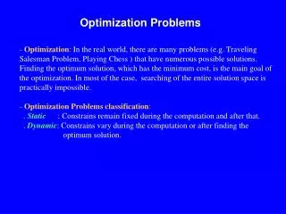
Linear programming minimize/maximize a linear function under equality/inequality linear constraints • Standard form: • The region satisfying all the constraints is the feasible region and it is convex
Linear programming (cont.) • The number of corner points is finite • The global maximum is at the corner point in which Z(x) is greater or equal to the value of Z at all adjacent corner points • The simplex method (Dantzig 1948) starts at a feasible corner point and visited a sequence of corner points until a maximum is obtained • #of iterations is almost always O(M) or O(N) whichever is larger, but can become exponential for pathological cases
The basic mechanism of the simplex method: A simple example • Standard form without equality constraints • Start at the origin: always a feasible corner point • N=2 , M=3 at most 10 corner points, but only 5 are feasible • at (x1,x2)=(0,0) the two last constraints intersect
The basic mechanism of the simplex method: A simple example • Add slack variables which transform inequality constraints to equality constraints • Start at the origin: (x1,x2,s1,s2,s3)=(0,0,2,3,4) , Z=0 • move to another corner point by letting, say, x1 grow • x1 maygrow until it hits another corner point, in which a different constraint holds => setting some si=0
The basic mechanism of the simplex method: A simple example • Divide all variables into two groups: basic/nonbasic • At the origin: (x1,x2,s1,s2,s3)=(0,0,2,3,4) • Choose a nonbasic that maximizes Z: x1 , this is the entering basic variable • x1 is increased until it hits the constraint • There, x1=2 => s1=0 and this is the leaving basic variable • At (2,0): (x1,x2,s1,s2,s3)=(2,0,0,3,4), Z=30 • Update the equations and continue untilno further increase in Z is available • Automatic exchange of variables: Simplex Tableau
Simplex Tableau with inequality constraints In proper form: • Exactly 1 basic variable per equation • The coefficient of each basic variable is 1 and this is the only non zero entry in its column • The RHS reveal the values of all basic variables • The entering basic variable has the most negative entry in the 0th row (for the objective Z) • The leaving basic variable is the one that minimizes RHS/coefficient of entering variable • Set the pivot to 1 and use it to eliminate all other non zeros in its column • The maximum is achieved when the 0th row 0
nonbasic =0 basic Slack variables s1 s2 s3 s1 s2 s3
Minimum Ratio Test entering basic leaving basic
Simplex Tableau with inequality (‘less than’), equality and ‘greater than’ constraints If an equality constraints are involved, e.g., x1+x2=4 • The origin is not feasible • Add an artificial variable to each equality constraint: x1+x2+t1=4 If a constraint is with ‘greater than’ sign: 3x1+2x2 16 • The origin is not feasible • Add a slack variable and an artificial variable to each ‘greater than’ constraint: 3x1+2x2-s1+t1=16 • In order to find a starting feasible corner point for the original LP, solve a Phase 1 LP in which the objective is to minimize the sum of all artificial variables: minimize Sti until all ti=0 =>feasible for the original LP
Simplex Tableau in general A general LP problem involves: • N original variables • Lless than constraints • Eequality constraints • G greater than constraints • Add L+G slack variables • Add E+Gartificial variables • To find a starting feasible corner point for LP, solve a Phase 1 LP:minimize Sti(sum of artificial variables) • INFEASIBILE: if at the end of Phase 1 Sti>0 • If Sti=0 continue to solve the original LP • UNBOUNDED: an entering basic variable is unlimited
Linear programming • The Simplex method: small and large problems • Interior point methods: very large problems (Karmarker 1984, polynomial-time algorithm) • Within ML should not exceed 100 variables • Many available software: MATLAB, numerical recipes,… • Adjust your problem to the used software • Linearization of both the energy functional and the constraints: the placement problem under pair wise non-overlap constraints
Exc#6: Window relaxation for the graph drawing problem Consider the following window W of 3x3 squares containing the nodes m,n and p: m is of size 1x1 located at (2,2); n is of size 0.8x0.8 located at (3.4,3.2); p is of size 0.5x0.5 located at (2.5,3). Find a correction to the locations of m,n and p such that the quadratic energy is minimized subject to inequality constraint demands that the area of nodes at each square <= 0.3 (4,4) (5,4) 8 4 7 9 1 n p 4 3 (0.5,1.5) 2 5 6 m 1 2 3 (1,1)
Calculate the current amount of nodes’ area present in each of the 9 squares • Calculate amkx e: the change (per unit length) in the amount of nodes’ area induced by a small change in the x direction of node m to square k, k=1,…,9. Similarly calculate amky ,ankx ,anky ,apkx and apky • Write the quadratic energy E as a function of the corrections to the variables in W • Calculate the current value of E • Write the 9 inequalities constraints associated with each square • Choose the active set of constraints and write the Lagrangian • Calculate the resulting system of equations and solve it • Does the solution seem to be reasonable? • Choose .25 of the solution, does E decrease at that point? • Write the linear programming formulation
Exc#6: Window relaxation for the graph drawing problem • Given a graph which is initially drawn at • Introduce a grid of mxm squares, each square of size hx by hy • Pick a window W of squares • Define by akix (akiy) the change in the total area in the k’th square per small change in 1. How should akix (akiy) be calculated 2. Write the quadratic energy minimization problem under equidensity constraints in W 3. Write the resulting linear system of equations 4. Write a linear programming formulation