Optimization Problems
Discover application of dynamic programming for optimization problems, analyzing techniques like greedy algorithms. Learn about matrix multiplication optimization and algorithms.


Optimization Problems
E N D
Presentation Transcript
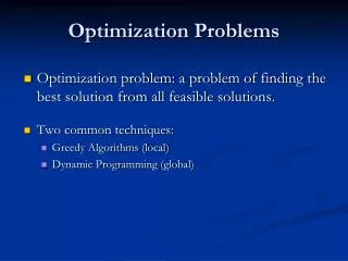
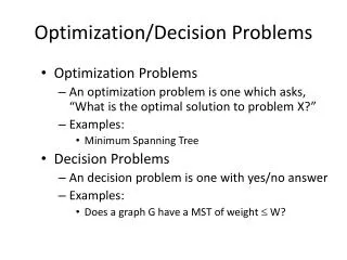
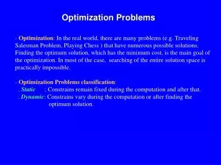
Optimization Problems • In which a set of choices must be made in order to arrive at an optimal (min/max) solution, subject to some constraints. (There may be several solutions to achieve an optimal value.) • Two common techniques: • Dynamic Programming (global) • Greedy Algorithms (local) Lin/Manocha/Foskey
Dynamic Programming • Similar to divide-and-conquer, it breaks problems down into smaller problems that are solved recursively. • In contrast, DP is applicable when the sub-problems are not independent, i.e. when sub-problems share sub-sub-problems. It solves every sub-sub-problem just once and save the results in a table to avoid duplicated computation. Lin/Manocha/Foskey
Elements of DP Algorithms • Sub-structure: decompose problem into smaller sub-problems. Express the solution of the original problem in terms of solutions for smaller problems. • Table-structure: Store the answers to the sub-problem in a table, because sub-problem solutions may be used many times. • Bottom-up computation: combine solutions on smaller sub-problems to solve larger sub-problems, and eventually arrive at a solution to the complete problem. Lin/Manocha/Foskey
Applicability to Optimization Problems • Optimal sub-structure (principle of optimality): for the global problem to be solved optimally, each sub-problem should be solved optimally. This is often violated due to sub-problem overlaps. Often by being “less optimal” on one problem, we may make a big savings on another sub-problem. • Small number of sub-problems:Many NP-hard problems can be formulated as DP problems, but these formulations are not efficient, because the number of sub-problems is exponentially large. Ideally, the number of sub-problems should be at most a polynomial number. Lin/Manocha/Foskey
Optimized Chain Operations • Determine the optimal sequence for performing a series of operations. (the general class of the problem is important in compiler design for code optimization & in databases for query optimization) • For example: given a series of matrices: A1…An , we can “parenthesize” this expression however we like, since matrix multiplication is associative (but not commutative). • Multiply a p x q matrix A times a q x r matrix B, the result will be a p x r matrix C. (# of columns of A must be equal to # of rows of B.) Lin/Manocha/Foskey
Matrix Multiplication • In particular for 1 i p and 1 j r, C[i, j] = k = 1 to qA[i, k]B[k, j] • Observe that there are pr total entries in C and each takes O(q) time to compute, thus the total time to multiply 2 matrices is pqr. Lin/Manocha/Foskey
Chain Matrix Multiplication • Given a sequence of matrices A1 A2…An , and dimensions p0 p1…pn where Ai is of dimension pi-1 x pi , determine multiplication sequence that minimizes the number of operations. • This algorithm does not perform the multiplication, it just figures out the best order in which to perform the multiplication. Lin/Manocha/Foskey
Example: CMM • Consider 3 matrices: A1be 5 x 4, A2be 4 x 6, and A3 be 6 x 2. Mult[((A1 A2)A3)] = (5x4x6) + (5x6x2) = 180 Mult[(A1 (A2A3 ))] = (4x6x2) + (5x4x2) = 88 Even for this small example, considerable savings can be achieved by reordering the evaluation sequence. Lin/Manocha/Foskey
Naive Algorithm • If we have just 1 item, then there is only one way to parenthesize. If we have n items, then there are n-1 places where you could break the list with the outermost pair of parentheses, namely just after the first item, just after the 2nd item, etc. and just after the (n-1)th item. • When we split just after the kth item, we create two sub-lists to be parenthesized, one with k items and the other with n-k items. Then we consider all ways of parenthesizing these. If there are Lways to parenthesize the left sub-list, R ways to parenthesize the right sub-list, then the total possibilities is LR. Lin/Manocha/Foskey
Cost of Naive Algorithm • The number of different ways of parenthesizing n items is P(n) = 1, if n = 1 P(n) = k = 1 to n-1P(k)P(n-k), if n 2 • This is related to Catalan numbers (which in turn is related to the number of different binary trees on n nodes). Specifically P(n) = C(n-1). C(n) = (1/(n+1))C(2n, n) (4n / n3/2) where C(2n, n) stands for the number of various ways to choosenitems out of2nitems total. Lin/Manocha/Foskey
DP Solution (I) • Let Ai…j be the product of matrices i through j. Ai…j is a pi-1 x pj matrix. At the highest level, we are multiplying two matrices together. That is, for any k, 1 k n-1, A1…n = (A1…k)(Ak+1…n) • The problem of determining the optimal sequence of multiplication is broken up into 2 parts: • : How do we decide where to split the chain (what k)? A : Consider all possible values of k. • : How do we parenthesize the subchains A1…k & Ak+1…n? A : Solve by recursively applying the same scheme. NOTE: this problem satisfies the “principle of optimality”. • Next, we store the solutions to the sub-problems in a table and build the table in a bottom-up manner. Lin/Manocha/Foskey
DP Solution (II) • For 1 i j n, let m[i, j] denote the minimum number of multiplications needed to compute Ai…j. • Example: Minimum number of multiplies for A3…7 • In terms of pi , the product A3…7 has dimensions ____. Lin/Manocha/Foskey
DP Solution (III) • The optimal cost can be described be as follows: • i = j the sequence contains only 1 matrix, so m[i, j]=0. • i < j This can be split by considering each k, i k < j, as Ai…k (pi-1 x pk ) times Ak+1…j (pk x pj). • This suggests the following recursive rule for computing m[i, j]: m[i, i] = 0 m[i, j] = mini k < j(m[i, k] + m[k+1, j] + pi-1pkpj ) for i < j Lin/Manocha/Foskey
Computing m[i, j] • For a specific k,(Ai …Ak)(Ak+1…Aj) = m[i, j] = mini k < j(m[i, k] + m[k+1, j] + pi-1pkpj ) Lin/Manocha/Foskey
Computing m[i, j] • For a specific k,(Ai …Ak)(Ak+1…Aj) = Ai…k(Ak+1…Aj) (m[i, k] mults) m[i, j] = mini k < j(m[i, k] + m[k+1, j] + pi-1pkpj ) Lin/Manocha/Foskey
Computing m[i, j] • For a specific k,(Ai …Ak)(Ak+1…Aj) = Ai…k(Ak+1…Aj) (m[i, k] mults) = Ai…kAk+1…j(m[k+1, j] mults) m[i, j] = mini k < j(m[i, k] + m[k+1, j] + pi-1pkpj ) Lin/Manocha/Foskey
Computing m[i, j] • For a specific k,(Ai …Ak)(Ak+1…Aj) = Ai…k(Ak+1…Aj) (m[i, k] mults) = Ai…kAk+1…j(m[k+1, j] mults) = Ai…j(pi-1pk pjmults) m[i, j] = mini k < j(m[i, k] + m[k+1, j] + pi-1pkpj ) Lin/Manocha/Foskey
Computing m[i, j] • For a specific k,(Ai …Ak)(Ak+1…Aj) = Ai…k(Ak+1…Aj) (m[i, k] mults) = Ai…kAk+1…j(m[k+1, j] mults) = Ai…j(pi-1pk pjmults) • For solution, evaluate for all k and take minimum. m[i, j] = mini k < j(m[i, k] + m[k+1, j] + pi-1pkpj ) Lin/Manocha/Foskey
Matrix-Chain-Order(p) 1. n length[p] - 1 2. for i 1 to n // initialization: O(n) time 3. do m[i, i] 0 4. for L 2 to n// L = length of sub-chain 5. dofor i 1 to n - L+1 6. do j i + L - 1 7. m[i, j] 8.for k i to j - 1 9. do q m[i, k] + m[k+1, j] + pi-1 pk pj 10. if q < m[i, j] 11. then m[i, j] q 12. s[i, j] k 13. return m and s Lin/Manocha/Foskey
Analysis • The array s[i, j] is used to extract the actual sequence (see next). • There are 3 nested loops and each can iterate at most n times, so the total running time is (n3). Lin/Manocha/Foskey
Extracting Optimum Sequence • Leave a split marker indicating where the best split is (i.e. the value of k leading to minimum values of m[i, j]). We maintain a parallel array s[i, j] in which we store the value of k providing the optimal split. • If s[i, j] = k, the best way to multiply the sub-chain Ai…j is to first multiply the sub-chain Ai…k and then the sub-chain Ak+1…j, and finally multiply them together. Intuitively s[i, j] tells us what multiplication to perform last. We only need to store s[i, j] if we have at least 2 matrices & j > i. Lin/Manocha/Foskey
Mult (A, i, j) 1. if (j > i) 2. then k = s[i, j] 3. X = Mult(A, i, k) // X = A[i]...A[k] 4. Y = Mult(A, k+1, j) // Y = A[k+1]...A[j] 5. return X*Y // Multiply X*Y 6. else returnA[i] // Return ith matrix Lin/Manocha/Foskey
Example: DP for CMM • The initial set of dimensions are <5, 4, 6, 2, 7>: we are multiplying A1 (5x4) times A2(4x6) times A3 (6x2) times A4 (2x7). Optimal sequence is (A1 (A2A3 )) A4. Lin/Manocha/Foskey
Finding a Recursive Solution • Figure out the “top-level” choice you have to make (e.g., where to split the list of matrices) • List the options for that decision • Each option should require smaller sub-problems to be solved • Recursive function is the minimum (or max) over all the options m[i, j] = mini k < j(m[i, k] + m[k+1, j] + pi-1pkpj ) Lin/Manocha/Foskey