Download
1 / 47
490 likes | 816 Views
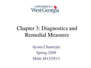
Chapter 3: Diagnostics and Remedial Measures. Ayona Chatterjee Spring 2008 Math 4813/5813. Validity of a regression model. Any one of the following features may not be appropriate. Linearity Normality of error terms. Important to examine the aptness of a model before making inferences.

E N D
Chapter 3: Diagnostics and Remedial Measures Ayona Chatterjee Spring 2008 Math 4813/5813
Validity of a regression model • Any one of the following features may not be appropriate. • Linearity • Normality of error terms. • Important to examine the aptness of a model before making inferences. • Consider diagnostic tools to justify the appropriateness of a mode. • Suggest remedial techniques to fix deviations.
Lets recall: A Dot Plot • A dotplot displays a dot for each observation along a number line. If there are multiple occurrences of an observation, or if observations are too close together, then dots will be stacked vertically. If there are too many points to fit vertically in the graph, then each dot may represent more than one point.
Stem and Leaf Diagram • In a stem-and-leaf plot each data value is split into a "stem" and a "leaf". The "leaf" is usually the last digit of the number and the other digits to the left of the "leaf" form the "stem".
Box Plot • Uses the max, minimum and the quartiles to plot the data. • Can draw conclusions about symmetry and outliers.
Time Series Plot • Also called sequence plot. • Used when data are collected in series over time. • Used to draw inference about patterns with time. • Seasonal or weekly effects.
Diagnostics for Predictor Variable • Let us look at the Toluca Company example given in chapter 1. • The predictor variable X was the lot size. • A dot plot, time series plot, stem and leaf plot and box pot for the data were obtained.
1 2 0 4 3 000 6 4 05 8 5 00 11 6 000 (3) 7 555 10 8 00005 5 9 5 10 00 3 11 00 1 12 5
Residuals • Residuals are the difference between the observed and predicted responses (Y). • For the normal error regression model, we assume that the error term is normally distributed. • If the model is appropriate for the data, this should be reflected in the residuals.
Departures from Model to be Studied by Residuals • The regression function is not linear. • The error terms do not have constant variance. • The error terms are not independent. • The model fits all but one or few outliers, • The error terms are not normally distributed. • One or several important predictor(s) have been omitted from the model.
Diagnostics for Residuals • Six diagnostic plots to judge departure from the simple linear regression model. • Plot of residuals against predictor variable. • The plot should have a random scatter of plots. • Plot of absolute or squared residuals against X. • Plot of residuals against the fitted values.
Diagnostics for Residuals • Plot of residuals against time or other sequence. • Should not display any trends. • Plots of residuals against omitted predictor variables. • Box plot of residuals. • Normal probability plot of residuals. • Should lie along a straight line.
Good Looking Plots Predictor
A example to study the relation between maps distributed and bus rider ship in eight cities. Here X is the # of bus transit maps distributed for free to residents at the beginning of the test period and Y is the increase during the test period in average daily busy rider ship during non peak hours. Nonlinearity of Regression Function X Y 80 0.60 220 6.70 140 5.30 120 4.00 180 6.55 100 2.15 200 6.60 160 5.75
Plots • Here a linear function appears to give a decent fit to the data set introduced in the previous slide. The regression equation obtained is • Y = -1.82 + 0.0435 X
Residual Plot • Here the departure from linearity if more visible as the residuals depart from 0 in a systematic manner. • The residual against the predictor is the preferred plot to judge linearity.
Nonconstancy or error variance • Here we have a residual plot against age for a study of the relation between blood pressure of adult women and their age, as age increases the residuals increase. In many business, social science and biological science, departure from constancy of error variance tends to be of the “megaphone” effect.
Nonconstancy of error variance • The two other types of departure from constant error variance are when we have a curvilinear regression function or the error variance increases over time.
Presence of outliers • Outliers are extreme observations and can be identified from box plot or dot plots. • Another option is to have a scatter plot of the semi-studentized residual • A rough rule of thumb in case of a large number of observations is to consider semi-studentized residuals with absolute value of 4 or more as outliers.
Example Here we can see that the scatter plot appears to have one outlier and this is pulling the regression line upwards. Thus in the residual plot we have so many observations in the lower half of the plot. Removing the outlier leads to a more uniformly linear scatter plot and better regression estimates.
Nonindependence of Error Terms • For time series data it is advised to plot residuals against time order. • This is to check if consecutive observations are independent of each other or not
Nonnormality of error terms • Large departures from normality is of concern. • A normal probability plot for the residuals in one way to judge normality.
Omission of Important Predictor Variables • Residuals should be plotted against variables omitted from the model that may have important effects on the response. • Example studies output Y and age of workers X.
Example • Lets work on the GPA data set. • Plot a box plot for the ACT scores, are there any noteworthy features in the plot? • Prepare a dot plot of the residuals. What information does this plot provide? • Plot the residuals against the fitted value. What departure from the regression model can be studied from this plot? What are your findings? • Prepare a normality plot of the residuals and comment on it.
Overview of Remedial Measures • If the linear regression model is not appropriate for your data set: • Abandon regression model and develop a new model. • Employ some transformation on the data so that the regression model is appropriate for the transformed data.
Nonlinearity of Regression Function • If the relation between X and Y is not linear, the following relations can be investigated: • Quadratic regression function. • Exponential regression function.
Transformations for Nonlinear Relation • To achieve linearity one can transform X or Y or both. • When the errors terms are normally distributed, we will transform X. • The following slide has some suggested transformations.
Prototype Transformation of X
Example 0.5 42.5 0.5 50.6 1 68.5 1 80.7 1.5 89.0 1.5 99.6 2 105.3 2 111.8 2.5 112.3 2.5 125.7 • Data from an experiment on the effect of number of days of training received X and performance Y in a battery of simulated sales situation are presented.
Transformation for Non-normality and Unequal Error variances • Unequal error variances and non-normality often occurs together. • To fix this we shall transform Y, since we need to change the shape and spread of the distribution for Y. • A simultaneous transformation on X may also be needed.
Prototype regression patterns Transformations on Y
Example: Plasma Levels • Using the data on plasma levels, • Draw a scatter plot of Age against plasma levels, comment on it. • Suggest a Suggest a suitable transformation. • Verify the validity of the transformation.
These plots supports the appropriateness of the linear regression model to the transformed data.
Box-Cox transformation • The Box-Cox procedure automatically identifies a transformation from the family of power transformations on Y. • The family of power transformations is of the form: • Here λ is a parameter to be determined from the data.
The new regression model • The normal error regression model with the response variable a member of the family of power transformations described in the previous slide is: • Along with the regression coefficients we now need to estimate λ. Most cases the maximum likelihood estimator of λ is obtained by conduction a numerical search in a potential range for λ.
Calculations for λ. • We standardize the responses so that the error magnitude does not depend on λ. • Once the standardized observations Wi have been obtained for a given λ value, they are regressed on the predictor variable X.
Example: Sales growth • A marketing researcher studied annual sales of a product that had been introduced 10 years ago. The data are as follows, where X is the year (coded) and Y is sales in thousands of units. Answer the following questions.
Prepare a scatter plot of the data. Does a linear relation appear adequate? • Use the Box-Cox procedure and standardization to find an appropriate power transformation of Y. Evaluate SSE for λ = 0.3, 0.4, 0.5, 0.6, 0.7. What transformation of Y is suggested?
X Y 0 98 1 135 2 162 3 178 4 221 5 232 6 283 7 300 8 374 9 395
Thus the regression equation using a square-root transformation on Y will give