Download
1 / 33
330 likes | 618 Views
Chapter 6 Diagnostics for Leverage and Influence. Ray-Bing Chen Institute of Statistics National University of Kaohsiung . 6.1 Important of Detecting Influential Observations. Usually assume equal weights for the observations. For example: sample mean

E N D
Chapter 6 Diagnostics for Leverage and Influence Ray-Bing Chen Institute of Statistics National University of Kaohsiung
6.1 Important of Detecting Influential Observations • Usually assume equal weights for the observations. For example: sample mean • In Section 2.7, the location of observations in x-space can play an important role in determining the regression coefficients (see Figure 2.6 and 2.7) • Outliers or observations that have the unusual y values. • In Section 4.4, the outliers can be identified by residuals
The point A is called leverage point. • Leverage point: • Has an unusual x-value and may control certain model properties. • This point does not effect the estimates of the regression coefficients, but it certainly will dramatic effect on the model summary statistics such as R2 and the standard errors of the regression coefficients.
Influence point: • For the point A, it has a moderately unusual x-coordinate, and the y value is unusual as well. • An influence point has a noticeable impact on the model coefficients in that it pulls the regression model in its direction. • Sometimes we find that a small subset of data exerts a disproportionate influence on the model coefficients and properties. • In the extreme case, the parameter estimates may depend on the influential subset of points than on the majority of the data.
We would like for a regression model to be representative of all of the sample observations, not an artifact of a few. • If the influence points are bad values, then they should be eliminated from the sample. • If they are not bad values, there may be nothing wrong with these points, but if they control key model properties we would like to know it, as it could affect the end use of the regression model. • Here we present several diagnostics for leverage and influence. And it is important to use these diagnostics in conjunction with the residual analysis techniques of Chapter 4.
6.2 Leverage • The location of points in x-space is potentially important in determining the properties of the regression model. • In particular, remote points potentially have disproportionate impact on the parameter estimates, standard error, predicted values, and model summary statistics.
Hat matrix plays an important role in identifying influential observations. H = X(X’X)-1X’ • H determines the variances and covariances of the fitted values and residuals, e. • The elements hij of H may be interpreted as the amount of leverage exerted by the ith observation yi on the ith fitted value.
The point A in Figure 6.1 will have a large hat diagonal and is assuredly a leverage point, but it has almost no effect on the regression coefficients because it lies almost on the line passing through the remaining observations. (Because the hat diagonals examine only the location of the observation in x-space) • Observations with large hat diagonals and large residuals are likely to be influential. • If 2p/n > 1, then the cutoff value does not apply.
Example 6.1 The Delivery Time Data • In Example 3.1, p=3, n=25. The cutoff value is 2p/n = 0.24. That is if hii exceeds 0.24, then the ith observation is a leverage point. • Observation 9 and 22 are leverage points. • See Figure 3.4 (the matrix of scatterplots), Figure 3.11 and Table 4.1 (the studentized residuals and R-student) • The corresponding residuals for the observation 22 are not unusually large. So it indicates that the observation 22 has little influence on the fitted model.
Both scaled residuals for the observation 9 are moderately large, suggesting that this observation may have moderate influence on the model.
6.3 Measures of Influence: Cook’s D • It is desirable to consider both the location of the point in x-space and the response variable in measuring influence. • Cook (1977, 1979) suggested to use a measure of the squared distance between the least-square estimate based on the estimate of the n points and the estimate obtained by deleting the ith point.
Usually • Points with large values of Di have considerable influence on the least-square estimate. • The magnitude of Di is usually assessed by comparing it to F, p, n-p. • If Di = F0.5, p, n-p, then deleting point I would move to the boundary an approximate 50% confidence region for based on the complete data set.
A large displacement indicates that the least-squares estimate is sensitive to the ith data point. • F0.5, p, n-p 1 • The Di statistic may be rewritten as • Di is proportional to the product of the square of the ith studentized residual and hii / (1 – hii). • This ratio can be shown to be the distance from the vector xi to the centroid of the remaining data. • Di is made up of a component that reflects how well the model fits the ith observation yi and a component that measures how far that points is from the rest of the data.
Either component (or both) may contribute to a large value of Di. • Di combines residual magnitude for the ith observation and the location of that point in x-space to assess influence. • Because , another way to write Cook’s distance measure is • Di is also the squared distance that the vector of fitted values moves when the ith observation is deleted.
Example 6.2 The delivery Time Data • Column b of Table 6.1 contains the values of Cook’s distance measure for the soft drink delivery time data.
6.4 Measure of Influence: DFFITS and DFBETAS • Cook’s D is a deletion diagnostic. • Blesley, Kuh and Welsch (1980) introduce two useful measures of deletion influence. • First one: How much the regression coefficient changes. • Here Cjj is the jth diagonal element of (X’X)-1
A large value of DFBETASj,i indicates that observation i has considerable influence on the jth regression coefficient. • Define R = (X’X)-1X’ • The n elements in the jth row of R produce the leverage that the n observations in the sample have on the estimate of the jth coefficient,
DFBETASj,i measures both leverage and the effect of a large residual. • Cutoff value: 2/n1/2 • That is if |DFBETASj,i| > 2/n1/2, then the ith observation warrant examination. • Second one: the deletion influence of the ith observation on the predicted or fitted value
DFFITSi is the number of standard deviation that the fitted value changes if observation i is removed. • DFFITSi is also affected by both leverage and prediction error. • Cutoff value: 2(pn)1/2
6.5 A Measure of Model Performance • The diagnostics Di, DFBETASj,i and DFFITSi provide insight about the effect of observations on the estimated coefficients and the fitted values. • No information about overall precision of estimation. • Generalized variance:
To express the role of the ith observation on the precision of estimation, we define • If COVRATIOi > 1, then the ith observation improves the precision of estimation. • If COVRATIOi < 1, inclusion of the ith point degrades precision.
Because of 1 / (1 – hii), a high-leverage point will make COVRATIOi large. • The ith point is considered influential if COVRATIOi > 1 + 3p/n or COVRATIOi < 1 – 3p/n • Theses cutoffs are only recommended for large sample. Example 6.4 The Delivery Time Data • The cutoffs are 1.36 and 0.64. • Observation 9 and 22 are influential. • Obs. 9 degrades precision of estimation. • The influence of Obs. 22 is fairly small.
6.6 Delecting Groups of Influential Observations • The above methods only focus on single-observation deletion diagnostics for influence and leverage. • Single-observation diagnostic => multiple-observation case. • Extend Cook’s distance measure • Let i be the m 1 vector of indices specifying the points to be deleted, and
Diis a multiple-observation version of Cook’s distance measure. • Large value of Diindicates that the set of m points are influential. • In some data sets, subsets of points are jointly influential but individual points are not! • Sebert, Montgomery and Rollier (1998) investigate the use of cluster analysisto find the set of influential observation in regression. (signle-linkage clustering procedure)
6.7 Treatment of Influential Observations • Diagnostics for leverage and influence are an important part of the regression model-builder’s arsenal of tools. • Offer the analyst insight about the data, and signal which observations may deserve more scrutiny. • Should influential observations ever be discarded? • A compromise between deleting an observation and retaining it is to consider using an estimation technique that is not impacted as severely by influential points as least squares.