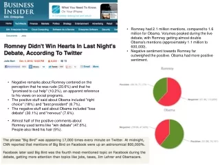
Analysis of Social Media Sentiment Towards Romney and Obama

1. Romney had 2.1 million mentions, compared to 1.6 million for Obama. Volumes peaked during the live debate, with Romney getting almost double Obama's mentions (approximately 1.1 million to 600,000). • Negative sentiment towards Romney far outweighed the positive. Obama had more positive sentiment. • Negative remarks about Romney centered on the perception that he was rude (20.6%) and that he "promised to cut help" (10.2%), an apparent reference to his views on social programs. • The positive stuff said about Obama included "right choice" (18%) and "best president" (8.7%). • The negative stuff said about Obama included "lose debate" (30.1%) and "nervous" (7.6%). • Almost half of the positive comments about Romney used terms like "win debate" (47.6%). People also liked his hair (9%).

2. Some review… http://www.colbertnation.com/the-colbert-report-videos/260955/january-07-2010/james-fowler

3. A question • Homophily: similar nodes ~= connected nodes • Which is cause and which is effect? • Do birds of a feather flock together? (Associative sorting) • Do you change your behavior based on the behavior of your peers? (Social contagion) • Note: Some authors use “homophily” only for associative sorting, some use it for observed correlation between attributes and connectivity.

5. Associative sorting example • Network: • 2D grid, each point connected to immediate neighbors, each point has color (red or blue) • Evolution: at each time t, each node will • Count colors of its neighbors • Move to a new (random) if it has <k neighbors of the same color • Typical result: strong spatial segregation, even with weak preferences k=3, Pr(red)=Pr(blue)=0.3

6. Social Contagion Example • Lots of different reasons behavior might spread • Fads, cascades, … • One reason: rational decisions made about products that have a “network effect” • I.e., the benefits and costs of the behavior are not completely local to the decision-maker • Example: PowerPoint, … • How can we analyze this? • From Easley & Kleinberg’s text, ch 16-17 • We’ll go into this more later on….

7. What if v is playing the game with many w’s ? If v has d neighbors and p*d of them choose A, then v should chose A iff pda>-(1-p)db ie, iff p>=b/(a+b)

8. Threshold: switch if 40% of neighbors switched

9. Threshold: switch if 40% of neighbors switched

10. General claim: dense clusters are less susceptible to cascades.

11. Thinking it through • Close-knit communities can halt a cascade of adoptions • Claim: a “complete cascade” happens iff there are no sufficiently close-knit clusters • A small increase in a/(a+b) might cause a big additional cascade. • Where the cascade starts might cause a big difference in the size of the cascade. • Marketing to specific individuals (e.g., in the middle of a cluster) might cause a cascade.

12. Thinking it Through • You cane extend this to cover other situations, e.g., backward compatibility: a-ε,b

13. A complicated example • NEJM, Christakis & Folwer, 2007: Spread of Obesity in A Large Social Network over 32 Years • Statistical model: for x connected to w: • obesity(x,t) = F(age(x), sex(x), …, obesity(x,t-1),obesity(w,t-1)) • Linear regression model, so you can determine influence of a particular variable • Looked at asymmetric links

14. Aside: linear regression • If true model for y is linear in x1, …, xn plus Gaussian noise then • regression coefficients are normally distributed • you can test to see if the influence of x is “real”

15. Another example • NEJM, Christakis & Fowler, 2007: Spread of Obesity in A Large Social Network over 32 Years • Statistical model: for x connected to w: • obesity(x,t) = F(age(x), sex(x), …, obesity(x,t-1),obesity(w,t-1)) • “Granger causality” • Linear regression model, so you can determine influence of a particular variable • But you’re tied to a parametric model and it’s assumptions • Looked at asymmetric links • Seems like a clever idea but … what’s the principle here?

17. Burglar Earthquake Alarm Phone Call The “Burglar Alarm” example • Your house has a twitchy burglar alarm that is also sometimes triggered by earthquakes. • Earth arguably doesn’t care whether your house is currently being burgled • While you are on vacation, one of your neighbors calls and tells you your home’s burglar alarm is ringing. Uh oh! • “A node is independent of its non-descendants given its parents” • “T wo nodes are independent unless they have a common unknown cause, are linked by an chain of unknown causes, or have a common known effect”

18. Causality and Graphical Models A: Stress A: Stress B: Smoking C: Cancer B: Smoking C: Cancer Pr(A,B,C)=Pr(C|B)Pr(B|A)Pr(A) Pr(A,B,C)=Pr(C|A)Pr(B|A)Pr(A)

21. Causality and Graphical Models A: Stress A: Stress B: Smoking C: Cancer B: Smoking C: Cancer Pr(A,B,C)=Pr(C|A)Pr(B|A)Pr(A) Pr(A,B,C)=Pr(C|B)Pr(B|A)Pr(A) • To estimate: • Pr(B=b) for b=0,1 • Pr(C=c|B=c) for b=0,1 and c=0,1 • To estimate: • Pr(B=b) for b=0,1 • Pr(C=c|B=c) for b=0,1 and c=0,1 The estimates for Pr(B) and Pr(C|B) are correct with either underlying model.

22. Causality and Graphical Models A: Stress A: Stress B: Smoking C: Cancer B: Smoking C: Cancer These two models are not “identifiable” from samples of (B,C) only. Def: A class of models is identifiable if you can learn the true parameters of any m in M from sufficiently many samples. Corr: A class of models M is not identifiable if there are some distributions generated by M that could have been generated by more than one model in M.

23. Causality and Graphical Models A: Stress A: Stress B: Smoking C: Cancer B: Smoking C: Cancer • How could you tell the models apart without seeing A? • Step 1: Interpret the arrows as “direct causality” • Step 2: Do a manipulation • Split the population into Sample and Control • Do something to make the Sample stop smoking • Watch and see if Cancer rates change in the Sample versus the control

24. A complicated example • NEJM, Christakis & Folwer, 2007: Spread of Obesity in A Large Social Network over 32 Years • Statistical model: for x connected to w: • obesity(x,t) = F(age(x), sex(x), …, obesity(x,t-1),obesity(w,t-1)) • Linear regression model, so you can determine influence of a particular variable • Looked at asymmetric links Not a clinical trial with an intervention

27. ??

28. d-separation • Fortunately, there is a relatively simple algorithm for determining whether two variables in a Bayesian network are conditionally independent: d-separation. • Definition: X and Z are d-separated by a set of evidence variables E iff every undirected path from X to Z is “blocked”, where a path is “blocked” iff one or more of the following conditions is true: ... ie. X and Z are dependent iff there exists an unblocked path

29. Y A path is “blocked” when... • There exists a variable Y on the path such that • it is in the evidence set E • the arcs putting Y in the path are “tail-to-tail” • Or, there exists a variable Y on the path such that • it is in the evidence set E • the arcs putting Y in the path are “tail-to-head” • Or, ... unknown “common causes” of X and Z impose dependency unknown “causal chains” connecting X an Z impose dependency Y

30. A path is “blocked” when… (the funky case) • … Or, there exists a variable V on the path such that • it is NOT in the evidence set E • neither are any of its descendants • the arcs putting Y on the path are “head-to-head” Known“common symptoms” of X and Z impose dependencies… X may “explain away” Z Y

31. ?? • “A node is independent of its non-descendants given its parents” • “T wo nodes are independent unless they have a common unknown cause or a common known effect”

32. ?? • Conclusion: • Y(j,t-1) influences Y(i,t) through latent homophily via the unblocked green path • There’s no way of telling this apart from the orange path (without parametric assumptions) – model is not “identifiable”

33. Some fixes Blocked at Z(j) ! (known intermediate cause) Blocked ! (known intermediate cause)

34. A consequence One can instantiate this model to show the same effects observed by Christakis and Fowler … even though there is no social contagion