CPC / NOAA: Satellite Rainfall Estimation and Applications for FEWS-NET

1. CPC / NOAA: Satellite Rainfall Estimation and Applications for FEWS-NET Nick Novella CPC / NCEP /NOAA Nicholas.Novella@noaa.gov NOAA / FEWS / Chemonics Training Session

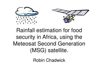
2. Satellite Rainfall Estimation • Purpose: • For a more complete spatial and temporal coverage for the monitoring of precipitation over the globe. • Implications: • It is germane for the monitoring of variability of weather and climate (operations & research) • Common Products within Community: • GPCP (NASA), CMAP (CPC) • TRMM (NASA) • CMORPH (CPC) • HydroEstimator (NESDIS) • TAMSAT (University of Reading, UK) • CHIRPS (USGS / UCSB)

3. Why is remote sensing needed?? • Station / gauge (in-situ) data: • Can be unreliable, inconsistent, poorly maintained. • Is subject to local quality control methods that can contribute to heterogeneity in dataset • Can not represent long-range spatial distribution of meteorological properties. • Is limited to land masses. • The character of precipitation differs greatly than other observations in meteorology • Discontinuous and Episodic (bounded quantity) • Greater need for constant coverage with consistent accuracy! • Offers insight to the shape/structure of meteorological disturbances that can produce significant rainfall. This is achieved by two fundamental classes of remote sensing: • Geostationary platform • Polar Orbiting platform

4. RFE : Rainfall Estimator • Inputs: • Gauge (GTS) • IR (GPI) • SSM / I (PM) • AMSU –B (PM) • Resolution: • Daily Analysis (06Z-06Z) • 0.1˚ gridded spatial resolution from 40S to 40N / -20W to 55E • 2001-present • Domains • Africa / SE Asia / Afghanistan

5. RFE Inputs: GTS • Data collected from rain gauges from a global network system of synoptic observations (GTS). • Provided by the World Meteorological Organization (WMO) • Data ingestion at CPC consists of: • Station extraction within each domain, routine QC methods, gridding via “Shepard” interpolation. • Approx. 2000 stations available for RFE • A variable number report daily (200-1000 stations) from 06Z – 06Z • Gauge data is the most accurate and “true” form of rainfall measurement, but suffers from aforementioned weaknesses... • Sparse coverage (e.g. 1 in 23,300 km2 gauge to area ratio across the African continent) • Errors / bias resulting from spatial interpolation

6. RFE Inputs: Infra-Red (GPI) • GOES Precipitation Index (GPI) based on IR temperatures from Geostationary satellites. • METEOSAT’s 2- 9 : centered at 0° Longitude • Imagery taken every ½ hour, with 48 snapshots daily • Spatial resolution of 0.05° / ~4km. • Given these attributes, GPI is the best capturer of the spatial distribution of rainfall. • Cloud Top Temperatures used as proxy to derive rainfall • Assumes monotonic relationship where rain intensity is proportional to the duration cloud top temperatures over a 24hr period. • Threshold temperature to define a cold cloud <= 235°K • Thus, the longer a cloud having temps below a threshold, the greater the rainfall • Caveats • GPI poor in mid and higher latitudes, underestimates rainfall from convective processes on fine scales. • Jet Streaks (cirrus)

7. RFE Inputs: SSM/I and AMSU-B • Special Sensor Microwave Imager (SSM/I), and Advanced Microwave Sounding Unit (AMSU-B) • Both derive daily rainfall totals from detecting upward scattering / emission of radiation associated with atmospheric water/ice. • Unlike IR, passive microwave (PM) sensors onboard polar-orbiting satellites (lower altitude ~1000km, orbital period ~100minutes) • Translates into decreased sampling frequency (poorer temporal & spatial coverage) • The tradeoff, however, is a more accurate, high resolution rainfall estimate, with exceptional performance associated with locally, intense convective rainfall.

8. RFE Inputs: Merging of all 4 inputs • Gridded GPI, SSM/I, AMSU-B and rain gauge analyses are computed to ascertain random error fields, and then reduced by maximum likelihood estimation methods (Xie & Arkin,1996). • In short, satellite-based estimates primarily are used to determine the “shape” of the rainfall distribution, while gauge-based estimates are used to quantify the “magnitude” of the rainfall distribution. • By doing so, final RFE estimates in close proximity to a station retain the value of the gauge report, and increasingly relies more on the satellite estimate as distance increases from that station. + + + = +

9. ARC2 : African Rainfall Climatology • Synopsis (CPC): • Used specifically for operational climate monitoring with meaningful anomalies based on a long-term satellite record. • Inputs: (a subset of the RFE) • Gauge (GTS) • IR (GPI) • Resolution: • Daily Analysis (06Z-06Z) • 0.1˚ gridded spatial resolution • 1983-present • Domains • Africa

10. RFE vs. ARC for FEWS • Why have two? …. First, lets compare estimators: • ARC well captures the spatial distribution of precipitation, but misses locally, intense rainfall due to the absence of PO MW inputs. • Question: If ARC is always drier than RFE, then why do we use it?

11. Answer: Because ARC2 is consistently dry, which lends itself to homogeneity in the long term precipitation time series. Attributed to the (GTS and IR) inputs. Raincurrent – Rainnormal = Anomaly Dry bias Dry bias No Dry Bias

12. Products: Satellite Rainfall Estimator Analyses • High resolution, daily rainfall data are easily aggregated into (totals / means) : Running Intervals (7,10,30,60,90,180-Day) • Dekadal (10-Day) Weekly • Monthly • Seasonal / Annual • These analyses are instrumental in illustrating short-term and long-term cycles of precipitation (e.g. ITCZ fluctuations, special event / monsoon totals)

13. Products: Satellite Rainfall Estimator Analyses • If a sufficient record length exists for satellite rainfall products, a rainfall climatology may be computed (e.g. ARC, now RFE): • Anomaly = Observed Rainfall ( for x period) minus Climatological Rainfall ( for x period) • Percent of Normal = Observed Rainfall ( for x period) / Climatological Rainfall ( for x period) * 100 - / = • These analyses are instrumental in illustrating both short-term / long-term trends of precipitation (e.g. flooding / drought) :

14. Percentile Anomaly • Rainfall percentile analyses place current anomaly fields in an historical context. • Suppose for a given gridpoint (i,j) during some period… 2015 = 150mm 2014 = 430mm 2013 = 560mm 2012 = 210mm …. 1983 = 440mm • These values are then ranked (sorted) to determine where 2015 falls with respect to all previous year’s rainfall. • perc(i,j) = (100/(nyr-0.5))*((nyr-rank+1)-0.5) perc(i,j) = 1.67

15. Rainfall Frequency: “Rain Days” • All rainfall estimate discussion has been based on the estimating/calculating the “magnitude” of rainfall (i.e. continuous quantity  [0:Inf] ) • What about the temporal behavior of rainfall? (i.e. discrete quantity) • Consider a hypothetical situation where a monsoonal area experiences nearly all of their normal total by early in the season. Following this extreme rainfall event, monsoonal rain virtually ceases causing a dry spell to negatively impact ground conditions for the remainder of the season. This may lead to misleading anomaly analyses. • To convert, we may define a “rain day” as some gridpoint (i,j) having received >= 1mm/day • Doing so for all of ARC2 will result in essentially a binary [0,1] dataset from 1983-present representing simply as either rain, or, no rain events. • We go back and compute current totals and climatology on this converted data to depict rain frequency.

16. Rainfall Frequency: “Consecutiveness” • A Discrete ARC2 [0,1] record may be used to determine “consecutiveness” of either wet/dry conditions. • Time scale may also be lengthened to weeks. This becomes quite useful for hazard criteria.

17. Seasonal Rainfall Performance Probability (SPP) • This new product quantitatively evaluates the probability of seasonal / sub-seasonal precipitation to finish at pre-defined anomaly thresholds over Africa. • Employs Kernel Density Estimate (KDE) methods to generate PDF’s of projected rainfall for the season based on ARC2 data by utilizing a daily long-term (1983-present) historical record of precipitation performances. • SPP is processed daily, and produces probability maps and point time series at a 0.1 degree resolution. • SPP enhances operational climate monitoring at CPC, which can translate into better decision making in food security, planning and response objectives for USAID/FEWS-NET. • < 25% of normal • < 50% of normal • < 80% of normal • 80% - 120% of normal • > 120% of normal

18. Observed Total @ Tc = 100mm • Climatological Total @ Tc = 150mm • % of Normal @ Tc = 66% • Climatological Total @ Tf= 500mm • Days Remaining in Season = 60 days Tc T0 Tf Mar 1, 2016 Apr 1, 2016 May 1, 2016 May 31, 2016 • Well.., 400mm of rain in 60 days is required for seasonal rains to reach “normal”, which works out to be a future prate of 6.66 mm/day from Tcto Tf. • Similarly, future prates, x, consisting of: • 0.42 mm/day is required to be at least 25% of normal • 2.50 mm/day is required to be at least 50% of normal • 5.00 mm/day is required to be at least 80% of normal • 6.66 mm/day is required to be at least 100% of normal • 8.33 mm/day is required to be at least 120% of normal • 10.8 mm/day is required to be at least 150% of normal • 15.0 mm/day is required to be at least 200% of normal • Based on the 30+ year history of observed prates, x(i) from Tcto Tf, how likely are these hypothetical prates, x, to happen in the future? • Solve KDE using x and x(i)to yield f(x). • Take integral to get CDF

19. Observed Total @ Tc = 100mm • Climatological Total @ Tc = 150mm • % of Normal @ Tc = 66% • Climatological Total @ Tf= 500mm • Days Remaining in Season = 60 days Tc T0 Tf Mar 1, 2016 Apr 1, 2016 May 1, 2016 May 31, 2016 • Well.., 400mm of rain in 60 days is required for seasonal rains to reach “normal”, which works out to be a future prate of 6.66 mm/day from Tc to Tf. • Similarly, future prates, x, consisting of: • 0.42 mm/day is required to be at least 25% of normal • 2.50 mm/day is required to be at least 50% of normal • 5.00 mm/day is required to be at least 80% of normal • 6.66 mm/day is required to be at least 100% of normal • 8.33 mm/day is required to be at least 120% of normal • 10.8 mm/day is required to be at least 150% of normal • 15.0 mm/day is required to be at least 200% of normal • Based on the 30+ year history of observed prates, x(i) from Tcto Tf, how likely are these hypothetical prates, x, to happen in the future? • Solve KDE using x and x(i) to yield f(x). • Take integral to get CDF • Plot critical prates for: • Below-Normal (<80% of normal) • Normal (80-120% of normal) • Above-Normal (>120% of normal) • This will then yield the respective probabilities for these anomaly categories by the end of the season.

20. Observed Total @ Tc = 100mm • Climatological Total @ Tc = 150mm • % of Normal @ Tc = 66% • Climatological Total @ Tf= 500mm • Days Remaining in Season = 60 days Tc T0 Tf Mar 1, 2016 Apr 1, 2016 May 1, 2016 May 31, 2016 • In this example, the persistence of below-normal rainfall is climatologically favored (~51%) over a seasonal recovery according to ARC2. • Historical precipitation exhibits a bimodal distribution, with greater density located in the 1st mode, and lesser density in the 2nd mode, for the remainder of the season. • Interestingly, the historical mean (5.83 mm/day  90% of Norm) is actually centered between the two modes in a PDF minima, suggesting either a wet/dry anomaly is more likely by end of season. • This example demonstrates how the rainfall climatology can create a more insightful outlook, rather than using the simple mean as a projection.

22. Application and Dissemination of NOAA products • Product Staging (http): http://www.cpc.ncep.noaa.gov/products/international/

23. Questions / Comments …?