Download
1 / 20
200 likes | 306 Views
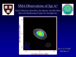
SMA Observations of Sgr A*. Dan P. Marrone, Ram Rao, Jim Moran, Jun-Hui Zhao Harvard-Smithsonian Center for Astrophysics. Sgr A * at 337 GHz 2004 May 25. Outline. Introduction to Sgr A*, submm perspective SMA Capabilities Observations of Sgr A* 2004: Polarimetry at 880 m ( 340 GHz)

E N D
SMA Observations of Sgr A* Dan P. Marrone, Ram Rao, Jim Moran, Jun-Hui Zhao Harvard-Smithsonian Center for Astrophysics Sgr A* at 337 GHz 2004 May 25
Outline • Introduction to Sgr A*, submm perspective • SMA Capabilities • Observations of Sgr A* • 2004: Polarimetry at 880m (340 GHz) • 2005: Photometry and polarimetry from 1.3 mm to 450 m
SMA What is known about Sgr A*? • Mass: 4 x 10⁶ M • From IR stellar orbits, VLBI proper motion monitoring • Luminosity: • ~1036 ergs/s ≈ 250L ≈ 10-8LEdd • Spectrum well measured from 90cm to 450m, NIR, X-ray • Peak in submillimeter, variable at all(?) wavelengths Sgr A* SED (Genzel et al. 2004)
What isn’t known? • Why is the luminosity so low? • Inefficient radiation and accretion – which model? • Jets and/or winds and/or convection and/or advection • Spectrum alone is insufficient to separate accretion models • Origin of the flares? • Connections to other sources: typical LLAGN?
New Tools - Variability • Multi-wavelength monitoring • Rapid changes require small radius • Direct connection to inner flow • Flare spectrum in submm/IR/X-ray should constrain mechanism(s) • (e.g. Liu, Petrosian & Melia 2004) • Recent results: • IR flares may show short periodicity, polarization (Genzel et al. 2003) • Coincident X-ray/IR/mm flares (Eckart et al. 2004, Zhao et al. 2004) • Need submm time resolution on timescales of flares (minutes) • Polarization information useful 1.65μm (H-band) flare (Genzel et al. 2004)
New Tools - Linear Polarization • Constrains density and B field through Rotation Measure: • RM can be used to infer inner • RM derived from PA measurement at multiple frequencies • Polarization only available in mm/submm (≤ 3.5mm) • No LP detected 21cm – 7mm • Polarization fraction measurementsrequire high resolution • SCUBA detection contaminated by surrounding emission • BIMA measurements …
Linear Polarization of Sgr A* • Confirmed interferometrically at 1.3mm (230 GHz) • (Bower et al. 2003, 2005) • LP is variable Need simultaneous data to infer RM • RM is low Need widely separated frequencies 230 GHz Polarization Fraction 230 GHz Position Angle Bower et al. (2005)
SMA – A New Observing Tool • The first dedicated submillimeter interferometer • 8 6-meter antennas on Mauna Kea • Sub-arcsecond resolution in three bands: • 1.3mm, 850, and 450 m (230, 345, 690 GHz) The Submillimeter Array (SMA)
New Capabilities from the SMA • High angular resolution eliminates JCMT confusion • Better sensitivity than BIMA: • Larger continuum bandwidth (2 vs. 0.8 GHz) • Better site: atmosphere and latitude • Allows precision photometry (10’ sampling), • polarization monitoring (sub-night sampling) • Wider frequency separation • Greater sideband separation than BIMA (10 vs. 2.8 GHz) • Simultaneous observations at multiple frequencies • Unprecedented sensitivity to RM
RM Sensitivity • Current Limit: ~106 rad/m2 • SMA single band observations: • 230 GHz RM = 1.1 x 10⁵ rad/m2/º • 340 GHz RM = 3.7 x 10⁵ rad/m2/º • 690 GHz RM = 3.1 x 10⁶ rad/m2/º • (BIMA at 230: 4.2 x 10⁵ rad/m2/º) • SMA dual band observations: • 230/690 RM = 1.1 x 10⁴ rad/m2/º • (For one 180º wrap: RM > 2x10⁶) RM detectible at < 105 rad/m2
SMA Polarimetry • Measurement of LP best done with CP feeds • Linear feeds mix I, Q, U • Circular feeds mix I, V (likely small), Q, U uncontaminated • SMA feeds are LP, single feed per band • Need polarization conversion, multiplexing scheme
LP to CP Conversion: Quarter-wave plates QWP LP CP Fast Axis Slow Axis (/4 retardation) Simple “Broadband” QWP: /4 at 3 03 /4 at 0, Perfect for 230/690 GHz
SMA Polarization Hardware Control computer Waveplate • Same observing technique as BIMA • Polarimetry at 230, 340, 690 GHz this year
Sgr A* Polarization at 340 GHz Q I U V
Polarization Fraction • P lower at 340 than 230 GHz • P varies significantly, unlike Bower et al. results at 230 GHz X-ray/IR Flare Data from: Aitken et al. (2000) Bower et al. (2003) Bower et al. (2005) Marrone et al. (2005, in prep)
Position Angle – Rotation Measure • If the 7/7 point is excluded (low S/N) • 20º PA shift from 1999 RM = 4 x 10⁵ rad/m2 • Matches changes seen at 230GHz • Consistent PA between sidebands (10 GHz separation) RM < 9 x 10⁵ rad/m2 All PA Data SMA Only
Accretion Rate Limits Accretion rate at large R ADAF, Bondi CDAF
222 GHz 684 GHz ν0.43 ν0.11 ~ν0 Sgr A* 230/690 GHz (continuum) T An et al., submitted
Upcoming Observations • 2005 GC observations are SMA Legacy Science • 3-band polarimetry (230/690 simultaneous) • First polarization measurement at 690 GHz (450m) • First detection of the RM • 5 coordinated monitoring nights • Chandra/VLT/Keck/SMA/VLA • Coordinated IR/submm polarization? • Precision short-timescale photometry • CP feeds: no effects from LP changes • Power spectra for comparison with accretion simulations • Time-resolved polarization measurements