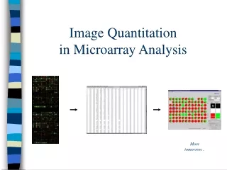
MicroArray Image Analysis
MicroArray Image Analysis. Robin Liechti ( robin.liechti@ie-bpv.unil.ch ) www.ch.embnet.org/CoursEMBnet/CHIP02/.../Liechti02_ images .ppt statwww.epfl.ch/davison/teaching/ Microarrays /lec/week04.ppt Mark Reimers (National Cancer Institute)


MicroArray Image Analysis
E N D
Presentation Transcript
MicroArray Image Analysis Robin Liechti (robin.liechti@ie-bpv.unil.ch) www.ch.embnet.org/CoursEMBnet/CHIP02/.../Liechti02_images.ppt statwww.epfl.ch/davison/teaching/Microarrays/lec/week04.ppt Mark Reimers (National Cancer Institute) www.ims.nus.edu.sg/Programs/microarray/files/MReimersTut1.ppt
Microarray analysis • Array construction, hybridisation, scanning • Quantitation of fluorescence signals • Data visualisation • Meta-analysis (clustering) • More visualisation
pseudo-colourimage sample(labelled) probe (on chip) [image from Jeremy Buhler] Technical
Images from scanner • Resolution • standard 10m [currently, max 5m] • 100m spot on chip = 10 pixels in diameter • Image format • TIFF (tagged image file format) 16 bit (65’536 levels of grey) • 1cm x 1cm image at 16 bit = 2Mb (uncompressed) • other formats exist e.g.. SCN (used at Stanford University) • Separate image for each fluorescent sample • channel 1, channel 2, etc.
Pseudo-color overlay cy3 cy5 Images : 2 color
Processing of images • Addressing or gridding • Assigning coordinates to each of the spots • Segmentation • Classification of pixels either as foreground or as background • Intensity extraction (for each spot) • Foreground fluorescence intensity pairs (R, G) • Background intensities • Quality measures
Affymetrix Image Reading • About 100 pixels per probe cell • Selects 16-25 brightest contiguous pixels • Take average of selected pixels • Variability in best pixels ~ 5-20% Image courtesy of Affymetrix
Probe Variation • Probes vary by two orders of magnitude on each chip Signal from 16 probes for the GAPDH gene on one chip • Individual probes don’t agree on fold changes • across chips • Bright probes more often, but not always, more reliable
Parameters to address the spots positions • Separation between rows and columns of grids • Individual translation of grids • Separation between rows and columns of spots within each grid • Small individual translation of spots • Overall position of the array in the image ScanAlyze Addressing (I) • The basic structure of the images is known (determined by the arrayer)
Addressing (II) • The measurement process depends on the addressing procedure • Addressing efficiency can be enhanced by allowing user intervention (slow!) • Most software systems now provide for both manual and automatic gridding procedures
Example from GenePix software http://transcriptome.ens.fr/sgdb/tools/download/image_analysis_en.pdf
Segmentation (I) • Classification of pixels as foreground or background -> fluorescence intensities are calculated for each spot as measure of transcript abundance • Production of a spot mask : set of foreground pixels for each spot
Segmentation (II) • Segmentation methods : • Fixed circle segmentation • Adaptive circle segmentation • Adaptive shape segmentation • Histogram segmentation
Bad example ! Fixed circle segmentation • Fits a circle with a constant diameter to all spots in the image • Easy to implement • The spots need to be of the same shape and size
Dapple finds spots by detecting edges of spots (second derivative) Adaptive circle segmentation • The circle diameter is estimated separately for each spot • Problematic if spot exhibits oval shapes
Adaptive shape segmentation • Specification of starting points or seeds • Regions grow outwards from the seed points preferentially according to the difference between a pixel’s value and the running mean of values in an adjoining region.
Bkgd Foreground Histogram segmentation • Uses a target mask chosen to be larger than any other spot • Foreground and background intensity are determined from the histogram of pixel values for pixels within the masked area • Example : QuantArray • Background : mean between 5th and 20th percentile • Foreground : mean between 80th and 95th percentile • Unstable when a large target mask is set to compensate for variation in spot size
Example from GenePix software http://transcriptome.ens.fr/sgdb/tools/download/image_analysis_en.pdf
Spot intensity • The total amount of hybridization for a spot is proportional to the total fluorescence at the spot • Spot intensity = sum of pixel intensities within the spot mask • Since later calculations are based on ratios between cy5 and cy3, we compute the average* pixel value over the spot mask *alternative : use ratios of medians instead of means
Background intensity • Motivation : spot’s measured intensity includes a contribution of non-specific hybridization and other chemicals on the glass • Fluorescence from regions not occupied by DNA should by different from regions occupied by DNA -> could be interesting to use local negative controls (spotted DNA that should not hybridize) • Different background methods :Local background, morphological opening, constant background, no adjustment
ScanAlyze ImaGene Spot, GenePix Local background • Focusing on small regions surrounding the spot mask. • Median of pixel values in this region • Most software package implement such an approach • By not considering the pixels immediately surrounding the spots, the background estimate is less sensitive to the performance of the segmentation procedure
Constant background • Global method which subtracts a constant background for all spots • Some findings suggests that the binding of fluorescent dyes to ‘negative control spots’ is lower than the binding to the glass slide • -> More meaningful to estimate background based on a set of negative control spots • If no negative control spots : approximation of the average background = third percentile of all the spot foreground values
No adjustment • Do not consider the background
References • Yang, Y. H., Buckley, M. J., Dudoit, S. and Speed, T. P. (2001), ‘Comparisons of methods for image analysis on cDNA microarray data’. Technical report #584, Department of Statistics, University of California, Berkeley. • Yang, Y. H., Buckley, M. J. and Speed, T. P. (2001), ‘Analysis of cDNA microarray images’. Briefings in bioinformatics, 2 (4), 341-349.
Next time • Data formats/files for Affymetrix microarrays • CEL and CDF • Intro to R • Reading in microarray data • Exploring array data • Assignment: • For the gene, Pbx1, determine the probe design on either the mouse Affymetrix 1.0 ST MoGene array or the Zebrafish genome array • ? What is the difference between a probe and a probeset? • You should be able to use resources at www.affymetrix.com but you might need to register to get access to data files.
For Pbx1, How many probes? What are the sequences of the probes? Where are the probes placed along the gene structure for Pbx1? Google Affymetrix web site