Chapter 7 Image Segmentation
Chapter 7 Image Segmentation. Chuan-Yu Chang ( 張傳育 )Ph.D. Dept. of Electronic Engineering National Yunlin University of Science & Technology chuanyu@yuntech.edu.tw Office: ES709 Tel: 05-5342601 Ext. 4337. Introduction.

Chapter 7 Image Segmentation
E N D
Presentation Transcript
Chapter 7 Image Segmentation Chuan-Yu Chang (張傳育)Ph.D. Dept. of Electronic Engineering National Yunlin University of Science & Technology chuanyu@yuntech.edu.tw Office: ES709 Tel: 05-5342601 Ext. 4337
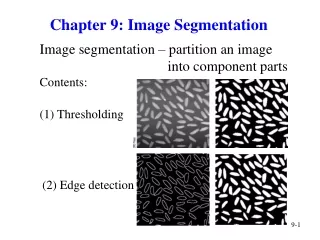
Introduction • Image segmentation refers to the process of partitioning an image into distinct regions by grouping together neighborhood pixels based on some pre-defined similarity criterion. • Segmentation is a pixel classification technique that allows the formation of regions of similarities in the image.
Introduction (cont.) • Image segmentation methods can be broadly classified into three categories: • Edge-based methods • The edge information is used to determine boundaries of objects. The boundaries are then analyzed and modified to form closed regions belonging to the objects in the image. • Pixel-based direct classification • Heuristics or estimation methods derived from the histogram statistics of the image are used to form closed regions belonging to the objects in the image. • Region-based methods • Pixels are analyzed directly for a region growing process based on a pre-defined similarity criterion to form closed regions belonging to the objects in the image.
Image Segmentation • Edge-Based Segmentation • Gray-level Thresholding • Pixel Clustering • Region Growing and Splitting • Artificial Neural Network • Model-Based Estimation
Edge-Based Segmentation • Edge-Based approaches • use a spatial filtering method to compute the first-order or second-order gradient information of the image. • Sobel, directional derivative masks can be used to compute gradient information of the image. • Laplacian mask can be used to compute second-order gradient information of the image. • For segmentation purpose • Edges need to be linked to form closed regions • Gradient information of the image is used to track and link relevant edges.
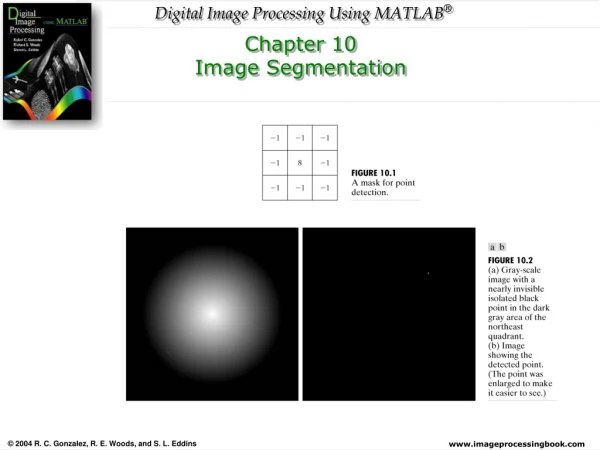
Introduction • Image segmentation algorithm generally are based on one of two basic properties of intensity values: • Discontinuity • Partition an image based on abrupt changes in intensity. • Similarity • Partitioning an image into regions that are similar according to a set of predefined criteria. • There are three basic types of gray-level discontinuities • Points, lines, and edges.
Detection of discontinuities • 最常用來偵測discontinuity的方法是對整張影像計算mask區域內的積之和(sum of product)
有小破洞 Detection of discontinuities • Point detection • 一個孤立的點,其灰階值一定和其周圍的點有相當明顯的差異。 取(c)圖最大灰階的90%作為threshold後的結果 Mask計算後的結果 飛機渦輪葉片的X光影像 T為非負值的Threshold
Detection of discontinuities • Line detection • 令R1, R2, R3, 及R4分別代表以下圖mask計算後的結果,如果影像中某點的|Ri|>|Rj|,則表示此點比較像第i種線條的方向。 • 若要偵測影像中某方向的線條時,可以該方向的mask進行運算,再取threshold後,留下的就是結果。
Detection of discontinuities • We are interested in finding all the lines that are one pixel thick and are oriented at -45. • Use the last mask shown in Fig. 10.3. 強度最強的line 偵測到的45度line
Detection of discontinuities • Edge detection • An edge is a set of connected pixels that lie on the boundary between two regions. • The “thickness” of the edge is determined by the length of the ramp. • Blurred edges tend to be thick and sharp edges tend to be thin.
Detection of discontinuities • The first derivative is positive at the points of transition into and out of the ramp as we move from left to right along the profile. • It is constant for points in the ramp, • It is zero in areas of constant gray level. • The second derivative is positive at the transition associated with the dark side of the edge, negative at the transition associated wit the light side of the edge, and zero along the ramp and in areas of constant gray level. 一階微分的大小可用來檢測是否存在邊界點, 二階微分的正負值可用來決定邊是在亮邊或暗邊。
Edge detection (cont.) • Two additional properties of the second derivative around an edge: • It produces two values for every edge in an image. • An imaginary straight line joining the extreme positive and negative values of the second derivative would cross zero near the midpoint of the edge. • The zero-crossing property of the second derivative is quit useful for locating the centers of thick edges.
Detection of discontinuities s=0 Image and gray-level profiles of a ramp edge • The entire transition from black to white is a single edge. First derivative image and the gray-level profile s=0.1 Second derivative image and the gray-level profile s=1 s=10
Edge detection (cont.) • The second derivative is even more sensitive to noise. • Image smoothing should be a serious consideration prior to the use of derivatives in applications . • Summaries of edge detection • To be classified as a meaningful edge point, the transition in gray level associated with that point has to be significant stronger than the background at that point. • Use a threshold to determine whether a value is “significant” or not. • We define a point in an image as being an edge point if its two dimensional first-order derivative is greater than a specified threshold. • A set of such points that are connected according to a predefined criterion of connectedness is by definition an edge. • Edge segmentation is used if the edge is short in relation to the dimensions of the image. • A key problem in segmentation is to assemble edge segmentations into linger edges. • If we elect to use the second-derivative to define the edge points in an image as the zero crossing of its second derivative.
Detection of discontinuities • Gradient operator • The gradient of an image f(x,y) at location (x,y) is defined as the vectorthe gradient vector points is the direction of maximum rate of change of f at coordinates (x,y). • The magnitude of the vector denoted ∇f, where • The direction of the gradient vector denoted by The angle is measured with respect to the x-axis.
Detection of discontinuities • Roberts operator • Gx=(z9-z5) • Gy=(z8-z6) • Prewitt operator • Gx=(z7+z8+z9)-(z1+z2+z3) • Gy=(z3+z6+z9)-(z1+z4+z7) • Sobel operator • Gx=(z7+2z8+z9)-(z1+2z2+z3) • Gy=(z3+2z6+z9)-(z1+2z4+z7)
Detection of discontinuities • 由於Eq.(10.1-4)的計算較耗時,因此梯度的計算通常以下式來近似: 用來偵測對角邊界的Prewitt及Sobel mask。
Detection of discontinuities Example 10-4 原始影像未smooth,造成一些細微的邊界點。 Fig. 10.10 shows the response of the two components of the gradient, |Gx| and |Gy|. The gradient image formed the sum of these two components.
Detection of discontinuities Example 10-4 原始影像經5*5 averaging filter ,移除細微的邊界點。
Detection of discontinuities Example 10-4 原始影像經Sobel 對角線邊界mask處理後的結果, 強化的45度角的邊界點。 • The horizontal and vertical Sobel masks respond about equally well to edges oriented in the minus and plus 45° direction. • If we emphasize edges along the diagonal directions, the one of the mask pairs in Fig. 10.9 should be used. • The absolute responses of the diagonal Sobel masks are shown in Fig. 10.12. • The stronger diagonal response of these masks is evident in these figures.
Detection of discontinuities • The Laplacian of a 2-D function f(x,y) is a second-order derivative defined as • For a 3x3 region, one of the two forms encountered most frequently in practice is (水平與垂直邊) • A digital approximation including the diagonal neighbors is given by (含水平、垂直、及對角邊)
Detection of discontinuities • 雖然Laplacian operator對於影像亮度的變化有反應,但因為下列缺點,仍很少應用在實際的邊界偵測: • 對雜訊太敏感 • 產生雙邊緣 • 無法偵測出邊的方向 • 因此,Laplacian operator在影像分割的角色在於 • 使用過零點(zero-crossing)的特性找出邊緣的位置 • 幫助確定一個像素點是在暗側還是亮側。
Detection of discontinuities • Laplacian of a Gaussian (LoG) • The Laplacian is combined with smoothing as a precursor to finding edges via zero-crossing, consider the functionwhere r2=x2+y2 and s is the standard deviation. • Convolving this function with an image blurs the image, with the degree of blurring being determined by the value of s. • The Laplacian of h is • The function is commonly referred to as the “Laplacian of a Gaussian” (LoG), sometimes is called the ”Mexican hat” function
Detection of discontinuities LoG中,Gaussian函數的目的在於smooth影像,而Laplacian運算子則以ZC來找出邊的位置。
Detection of discontinuities • Comparing Figs/ 10.15(b) and (g) • The edges in the zero-crossing image are thinner than the gradient edges. • The edges determined by zero-crossings form numbers closed loops. • “spaghetti effect” is one of the most serious drawbacks of this method. • The major drawback is the computation of zero crossing.
Detection of discontinuities ZC的偵測,可將LoG中的正值設為白色, 負值設為黑色,以得到近似的結果。 Gradient edge與LoG edge的差異: 1. ZC的邊比gradient的邊細。 2. ZC的邊有義大利麵的現象發生, (region化) 3. ZC的計算量相當大
Edge Linking and Boundary Detection • Edge detection的目的在於找出邊界上的點,但這些點很可能會有斷裂的現象,因此需要邊的連接(edge linking) 來將邊界點組合成有意義的邊界。 • Edge linking • Based on pixel-by-pixel search to find connectivity among the edge segmentations. • The connectivity can be defined using a similarity criterion among edge pixels. • Local Processing • 分析每個被標記為邊界點的pixel在一個小區域(3x3, 5x5)的特徵,把所有相似的點連接起來,這些具有相似特性的像素點就形成了邊界。 • 建立邊界點相似性的兩個主要特性: • 用來產生邊界點的梯度運算子反應的強度,Eq.(10.1-4) • 梯度向量的方向, Eq. (10.1-5)
Edge Linking and Boundary Detection • 像素點(x,y)和(x0,y0)的梯度相似性 • 像素點(x,y)和(x0,y0)的梯度角度相似性 • 如果上面兩個條件均滿足,則將(x0,y0)與(x,y)連接起來。
Edge Linking and Boundary Detection • Example 10-6: the objective is to find rectangles whose sizes makes them suitable candidates for license plates. • The formation of these rectangles can be accomplished by detecting strong horizontal and vertical edges. • Linking all points, that had a gradient value greater than 25 and whose gradient directions did not differ by more than 15°. 使用垂直的Sobel operator 分別對圖(b)及(c)進行edge linking的動作,將梯度大於25,且角度小於15度的點連起來。 使用水平的Sobel operator
Boundary Tracking • A* search algorithm • Select an edge pixel as the start node of the boundary and put all of the successor boundary pixels in a list, OPEN • If there is no node in the OPEN list, stop; otherwise continue. • For all nodes in the OPEN list, compute the cost function t(z) and select the node z with the smallest cost t(z). Remove the node z from the OPEN list and label it as CLOSED. The cost function t(z) may be computed as
Boundary Tracking (cont.) • If z is the end node, exit with the solution path by tracking the pointers; otherwise continue. • Expand the node z by finding all successors of z. If there is no successor , goto Step 2; otherwise continue. • If a successor zi is not labeled yet in any list, put it in the list OPEN with updated cost asc(zi)=c(z)+s(z, zi)+d(zi) and a pointer to its predecessor z. • If a successor zi is already labeled as CLOSED or OPEN, update its value by c’(zi)=min[c(zi),c(z)+s(z,zi)]Put those CLOSED successors whose cost function x’(zi) s were lowered, in the OPEN list and redirect to z the pointers from all nodes whose cost were lowered. Goto Step 2.
End Node Start Node Boundary Tracking (cont.) • Figure 7.1. Top: An edge map with magnitude and direction information; Bottom: A graph derived from the edge map with a minimum cost path (darker arrows) between the start and end nodes.
在xy平面上,a’表通過(xi, yi)和(xj, yj)的直線,b’表截距 Edge Linking and Boundary Detection • Global Processing via the Hough Transform • 點是否被連接,端視該點是否處於一特定形狀的曲線而定。
Edge Linking and Boundary Detection • Hough Transform • 將參數空間細分成accumulator cell • 一開始所有的accumulator cell均設為0 • 對影像上的每一點(xk,yk) ,將參數a設成a軸上每一個允許的細分值,用等式b=-xka+yk計算對應的b值。 • 將得到的b值化整到最近的b軸 • 若ap的結果為bq,則A(p,q)=A(p,q)+1
Edge Linking and Boundary Detection • 當直線趨近垂直時,斜率趨近無窮大,因此將直線方程式改以下式表示:
Edge Linking and Boundary Detection X, Y平面上五個點(1, 2, 3, 4, 5) ,在rq平面的曲線 X, Y平面上有五個點(1, 2, 3, 4, 5) 從交點A知道, 點1, 3, 5)共線。 交點B表示點2,3,4共線
Edge Linking and Boundary Detection • Edge-linking based on Hough transform • 計算影像的梯度,並取threshold以得到binary image。 • 訂出rq平面的範圍。 • 對二元化影像進行Hough Transform。 • 檢查accumulator cell中較高的值 • 依其對應的rq找出直線。
Edge Linking and Boundary Detection Sobel的結果跑道有斷格 空中紅外線影像,有兩個停機坪及跑道 Hough Transform結果 從accumulator cells 中找出前三大值
q p Edge Linking and Boundary Detection • Global Processing via Graph-Theoretic Techniques • 將邊界點的線段以圖形法表示,找尋最低成本的路徑來代表重要的邊界。 • 此法在雜訊影像中有不錯的效果。但演算法複雜、耗時。 • Graph G=(N,U) • N: node的集合 • U: N的元素對集合 • U的元素(ni,nj)對稱為arc,ni,稱為parent, nj稱為successor。 • 確認successor的過程稱為expansion。 • Level 0只有一個點稱為start或root。最後的level稱為goal。 • Cost (ni,nj)為每個arc的成本 • 一序列的節點稱為路徑(path) • n1到nk的Path成本(cost)定義成
Edge Linking and Boundary Detection 每一個edge element定義成 成本 座標 灰階值 其中,H為影像中最大的灰階值, f(x)為x點的灰階值
Edge Linking and Boundary Detection • By convention, the point p is on the right-hand side of the direction of travel along edge elements. • To simplify, we assume that edges start in the top row and terminate in the last row. • p and q are 4-neighbors. • An arc exists between two nodes if the two corresponding edge elements taken in succession can be part of an edge. • The minimum cost path is shown dashed. • Let r(n) be an estimate of the cost of a minimum-cost path from s to n plus an estimate of the cost of that path from n to a goal node; • Here, g(n) can be chosen as the lowest-cost path from s to n found so far, and h(n) is obtained by using any variable heuristic information. (10.2-7)
Edge Linking and Boundary Detection • Graph search algorithm • Step1: Mark the start node OPEN and set g(s)=0. • Step 2: If no node is OPEN exit with failure; otherwise, continue. • Step 3: Mark CLOSE the OPEN node n whose estimate r(n) computed from Eq.(10.2-7) is smallest. • Step 4: If n is a goal node, exit with the solution path obtained by tracing back through the pointets; otherwise, continue. • Step 5: Expand node n, generating all of its successors (If there are no successors go to step 2) • Step 6: If a successor ni is not marked, set • Step 7: if a successor ni is marked CLOSED or OPEN, update its value by lettingMark OPEN those CLOSED successors whose g’ value were thus lowered and redirect to n the pointers from all nodes whose g’ values were lowered. Go to Step 2.
Edge Linking and Boundary Detection Example 10-9: noisy chromosome silhouette(有雜訊的染色體影像) The edge is shown in white, superimposed on the original image.
Thresholding • Thresholding • To select a threshold T, that separates the objects form the background. • Then any point (x,y) for which f(x,y)>T is called an object point; otherwise, the point is called a background point. • Multilevel thresholding • Classifies a point (x,y) as belonging to one object class ifT1 <f(x,y)≤T2, and to the other object class if f(x,y) >T2 • And to the background if f(x,y)≤T2
Thresholding • In general, segmentation problems requiring multiple thresholds are best solved using region growing methods. • The thresholding may be viewed as an operation that involves tests against a function T of the formwhere f(x,y) is the gray-level of point (x,y) and p(x,y) denotes some local property of this point. • A threshold image g(x,y) is defined as • Thus, pixels labeled 1 correspond to objects, whereas pixels labeled 0 correspond to the background. • When T depends only on f(x,y) the threshold is called global. If T depends on both f(x,y) and p(x,y), the threshold is called local. • If T depends on the spatial coordinates x and y, the threshold is called dynamic or adaptive.
The role of illumination • An image f(x,y) is formed as the product of a reflectance component r(x,y) and an illumination component i(x,y). • In ideal illumination, the reflective nature of objects and background could be easily separable. • However, the image resulting from poor illumination could be quit difficult to segment. • Taking the natural logarithm of Eq.(10.3-3) (10.3-4) (10.3-5)
The role of illumination • From probability theory, • If i’(x,y) and r’(x,y) are independent random variables, the histogram of z(x,y) is given by the convolution of the histograms of i’(x,y) and r’(x,y).
Pixel-based Direct Classification Methods 電腦產生的反射函數 電腦產生的照度函數 影像f(x,y)可看作是反射量r(x,y)和照度i(x,y)的乘積。 Fig. (a)*Fig(c) 物體和背景的反射特性,使她們容易被分割,但差的照明,會使產生的影像難以分割。