Download
1 / 29
290 likes | 365 Views
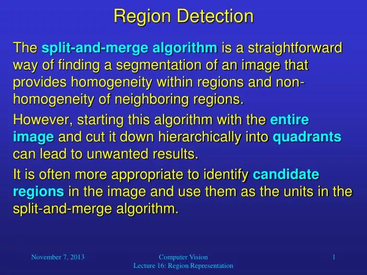
Region Detection. The split-and-merge algorithm is a straightforward way of finding a segmentation of an image that provides homogeneity within regions and non-homogeneity of neighboring regions.

E N D
Region Detection • The split-and-merge algorithm is a straightforward way of finding a segmentation of an image that provides homogeneity within regions and non-homogeneity of neighboring regions. • However, starting this algorithm with the entire image and cut it down hierarchically into quadrants can lead to unwanted results. • It is often more appropriate to identify candidate regions in the image and use them as the units in the split-and-merge algorithm. Computer Vision Lecture 16: Region Representation
Region Detection • Such candidate regions could be determined through variants of thresholding. • We will always speak of brightness thresholding, but other features such as texture or color could be used as well. • As you will see, prior knowledge about the scene can be helpful for correct region detection, such as • intensity characteristics of objects, • sizes of objects, • fraction of the image occupied by objects, or • number of different types of objects in the image. Computer Vision Lecture 16: Region Representation
P-Tile (Percentile) Method • If we have a good estimate for the proportion of the image occupied by objects, we can use the very simple P-Tile method. • This is possible, for example, in the case of optical character recognition, where the proportion of characters (objects) on a page does not vary a lot. • To set the threshold for separating objects and background, we first compute a histogram of the intensity values in the image. • Let us say that our estimate of the proportion of object pixels in the image is P%. Computer Vision Lecture 16: Region Representation
count (100 – P)% P% 0 T 255 intensity P-Tile (Percentile) Method • We set the threshold T so that P% of the pixels (area below the curve) have below-threshold intensity. • These will be classified as objects, and the other pixels will be classified as background. Computer Vision Lecture 16: Region Representation
Mode Method • If we cannot estimate the proportion of the image occupied by objects, then the P-Tile method cannot be applied. • However, if we know that the objects have approximately the same brightness which is different from the background brightness, we can use the Mode method. • Assuming that we have some Gaussian noise in our image, we expect our intensity histogram to be the sum of two normal distributions with parameters (1, 1) and (2, 2). Computer Vision Lecture 16: Region Representation
count 1 2 0 T 255 intensity P-Tile (Percentile) Method • The result is the histogram shown in red. • We would like to find the valley between the two peaks to set our threshold T. Computer Vision Lecture 16: Region Representation
Mode Method • Usually, the two peaks are not separated as clearly as in the previous example. • We need an appropriate algorithm to estimate the location of the valley between the two peaks. • A simple but powerful algorithm based on “peakiness detection” is given on the following slide. • It does not require a-priori information on any of the parameters 1, 1, 2 or 2. • We just have to set a value for the expected minimum intensity difference between the two peaks. Computer Vision Lecture 16: Region Representation
Peakiness Detection • Find two local maxima in the histogram H that are at some minimum distance apart. Suppose these occur at gray values gi and gj. • Find the lowest point gk in the histogram H between gi and gj. • Find the peakiness, defined as min[H(gi), H(gj)]/H(gk). Use smoothing before running the algorithm to avoid division by zero. • Find the combination (gi, gj, gk) with highest peakiness. Use the value gk as the threshold value to separate the objects from the background. Computer Vision Lecture 16: Region Representation
Peakiness Detection • This approach can easily be generalized to images with multiple objects having different intensity values. • For n such objects we need to determine n different thresholds T1, …, Tn. • T1 separates the background from the brightest object, T2 separates the brightest object from the second-brightest, and so on. • We can adapt our peakiness detection algorithm to estimate the optimal values for these thresholds. Computer Vision Lecture 16: Region Representation
Limitations of Histogram Methods • The main disadvantage of histogram methods is their disregard of spatial information. • Obviously, spatial information is important: Pixels of similar brightness are even more likely to belong to the same object when they are spatially close to each other (surface coherence). • Therefore, it is a good idea to use threshold methods in combination with spatial techniques such as split-and-merge. Computer Vision Lecture 16: Region Representation
Region Representation • Depending on the purpose of our system, we may want to represent the regions that we detected in a specific way. • There are three different basic classes of representation: • array representation, • hierarchical representation, and • symbolic representation. • We will now discuss these different approaches. Computer Vision Lecture 16: Region Representation
Array Representation • The simplest way to represent regions is to use a two-dimensional array of the same size as the original image. • Each entry indicates the label of the region to which the pixel belongs. • This technique is similar to the result of component labeling in binary images. • If we have overlapping regions, we can provide a mask for each region. • A mask is a binary array in which 1-pixels belong to the region in question and 0-pixels do not. Computer Vision Lecture 16: Region Representation
Hierarchical Representation • Hierarchical representation of images allows us to represent the visual information at multiple resolutions. • This is useful for a variety of tasks in computer vision. • For example, the presence and number of certain objects can be more efficiently detected at low resolution. • Then object identification can be performed at high resolution. • We will look at two techniques: pyramids and quad trees. Computer Vision Lecture 16: Region Representation
Pyramids • A pyramid is a set of pixel arrays, each of which shows the same image at a different resolution. • The level 0 image at the top of the pyramid consists of only 1 pixel. • Each successive level has twice as many pixels in x and y direction as the level above it. • Therefore, an n×n image is represented by levels0 to log2n. • The following slide shows the pyramid representation of a 512×512 image. Computer Vision Lecture 16: Region Representation
Pyramids Computer Vision Lecture 16: Region Representation
Quad Trees • Quad trees are a method for hierarchically representing binary images. • The root of a quad tree stands for the entire image, and its 4 children represent the 4 quadrants of the image. • If a quadrant is completely white or completely black, the corresponding node is marked white or black, respectively. • Otherwise, the node is expanded, and its children represent the quadrants within the original quadrant. • This process is repeated recursively until all pixels are represented. Computer Vision Lecture 16: Region Representation
Quad Trees Computer Vision Lecture 16: Region Representation
Symbolic Representation • For each region, represent information such as: • enclosing rectangle • moments • compactness • mean and variance of intensity • etc. • In other words, symbolic representation of a region means that we describe its characteristics using a set of (typically numerical or categorical) parameters. Computer Vision Lecture 16: Region Representation
Data Structures • How can we represent regions in computer programs? • We will look at two different approaches: Region adjacency graphs, picture trees, and super grids. • Region adjacency graphs are just undirected graphs, where each vertex represents a region. • The edges in the graph indicate which regions are adjacent to each other. Computer Vision Lecture 16: Region Representation
Region Adjacency Graphs Computer Vision Lecture 16: Region Representation
Picture Trees • Picture trees are a hierarchical structure for storing regions. • The rule for representation is the “is-included-in” relationship: • All child regions are included in their parent region. Computer Vision Lecture 16: Region Representation
Super Grids • If we want to represent region boundaries in an array, it is unclear to which region the pixels on the boundary belong (left: image; center: boundary). • If we expand our grid (right image), the boundary can be indicated without ambiguity. Computer Vision Lecture 16: Region Representation
Chain Codes • An interesting way of describing a contour is using chain codes. • A chain code is an ordered list of local orientations (directions) of a contour. • These local directions are given through the locations of neighboring pixels, so there are only eight different possibilities. • We assign each of these directions a code, e.g.: Computer Vision Lecture 16: Region Representation
Chain Codes • Then we start at the first edge in the list and go clockwise around the contour. • We add the code for each edge to a list, which becomes our chain code. Computer Vision Lecture 16: Region Representation
Chain Codes • What happens if in our chain code for a given contour we replace every code n with (n mod 8) + 1 ? • The contour will be rotated clockwise by 45 degrees. • We can also compute the derivative of a chain code, also referred to as difference code. • Difference codes are rotation-invariant descriptors of contours. • Some features of regions, such as their corners or areas, can be directly computed from chain or difference codes. Computer Vision Lecture 16: Region Representation
Slope Representation • The slope representation of a contour (also called the -s plot) is like a chain code for continuous data. • Along the contour, we plot the tangent versus arc length s. • Then horizontal line segments in the -s plot correspond to straight line segments in the contour. • Straight line segments at other orientations in the -s plot correspond to circular arcs in the contour. • Other segments in the -s plot correspond to other curve primitives in the contour. Computer Vision Lecture 16: Region Representation
Slope Representation • Note that in this plot not the actual arc length is used, but its horizontal projection: Computer Vision Lecture 16: Region Representation
Slope and Curvature Density Functions • The slope density function is the histogram of all slopes (tangent angles) in a contour. • This function can be used for recognizing objects. • We can also use the derivative of the slope representation, which we can call the curvature representation. • Its histogram is the curvature density function. • The curvature density function can also be used to recognize objects. • Its advantage is its rotation invariance, i.e., matching two curvature density functions determines similarity even if the two objects have different orientations. Computer Vision Lecture 16: Region Representation
90 180 0 Density Density Density Density 270 Square Diamond 0 0 0 0 90 90 90 90 180 180 180 180 270 270 270 270 360 360 360 360 Angle Angle Angle Angle Circle Ellipse Examples of Slope Density Functions Computer Vision Lecture 16: Region Representation