Download
1 / 16
160 likes | 430 Views
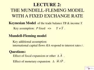
LECTURE 2: THE MUNDELL-FLEMING MODEL WITH A FIXED EXCHANGE RATE. Keynesian Model of the trade balance TB & income Y. Key assumption: P fixed => . Mundell-Fleming model

E N D
LECTURE 2:THE MUNDELL-FLEMING MODEL WITH A FIXED EXCHANGE RATE • Keynesian Model of the trade balance TB & income Y.Key assumption: P fixed => . • Mundell-Fleming model • Key additional assumption: international capital flows KA respond to interest rates i . • Questions: Effect of fiscal expansion or other .Effect of monetary expansion / .
ALTERNATE APPROACHES TO DETERMINATION OF EXTERNAL BALANCE • Elasticities Approach to the Trade Balance • Keynesian Approach to the Trade Balance • Mundell-Fleming Modelof theBalanceofPayments • Monetary Approach to the Balance of Payments • NonTraded Goods or Dependent-Economy Model of the Trade Balance • Intertemporal Approach to the Current Account
KEYNESIAN MODEL OF THETRADE BALANCE • Import demand is a function of the exchange rate & income. The same for exports: => TB = X(E,Y*) – IM(E,Y),where IM is here defined to be import spending expressed in domestic terms. • . • If the domestic country is small, Y* is exogenous; drop for simplicity. Rewrite TB = . Notationally, we embody all E effects (whether via exports or imports) in ; And we assume the Marshall-Lerner condition holds: .
Empirical estimates of sensitivity of exports and imports to E & Y • For empirical purposes, we estimate by OLS regression • with allowance for lags, giving J-curve; • controlling for income Y & Y* as well as E, • shown in logs, giving parameters as: • price elasticities & income elasticities. • Illustration: Marquez (2002) finds for most Asian countries: • Marshall-Lerner condition holds, after a couple of years, and • income elasticities are in the 1.0-2.0 range. log X
Estimated price elasticities (LR) satisfy the Marshall-Lerner Condition. Estimatedincome elasticities are mostly between1.0 - 2.0.
An application of the marginal propensity to import: Why did trade fall so much more sharply than income in the 2008-09 global recession? 2009 Bussière, Callegari, Ghironi, Sestieri, & N.Yamano, 2013,"Estimating Trade Elasticities: Demand Composition and the Trade Collapse of 2008-2009."
Why did trade fall so sharply in the 2008-09 global recession? Bussière, Callegari, Ghironi, Sestieri, & Yamano, 2013, "Estimating Trade Elasticities: Demand Composition and the Trade Collapse of 2008-09." The usual explanations involve trade credit, inventories, and trade in intermediate inputs.
Bussière et al (2013) argue that Investment, which declined much more in 2009 than the other components of GDP, has a higher marginal propensity to import than the other components. Behavior of real components of GDP in the 2008-09 recession GDP Demand, adjusted for import-intensity Imports & Exports Investment Bussière, Callegari, Ghironi, Sestieri, & N.Yamano,"Estimating Trade Elasticities: Demand Composition and the Trade Collapse of 2008-2009.“
Trade Balance = TB = (E) – mY. Aggregate output = domestic Aggregate Demand + net foreign demand:Y = A(i, Y) + TB(E, Y), More specifically, letA(i, Y) = Ā - b(i) + cY,where the function -b( ) captures the negative effect of the interest rate i on investment spending, consumer durables, etc. Solve to get the IS curve: where s 1 – c is the marginal propensity to save. where and . Combining equations, Y =
IS curve: An inverse relationship between i and Y consistent with the equilibrium that supply = demand in the goods market.
The Mundell-Fleming model introduces capital flows The overall balance of payments is given by BP = TB + KA , where , the degree of capital mobility > 0. We want to graph BP = 0. Solve for the interest rate: slope = m/
Finally, the LM curve is given by __ __M / P = L ( i, Y) where LM´ → A monetary expansion shifts the LM curve to the right .
Causes of Capital Flows to Emerging Markets • “Pull” Factors (internal causes) • 1. Monetary stabilization => LM shifts up • 2. Removal of capital controls => κ rises • 3. Spending boom => IS shifts out/up • 4. Domestic privatization, => IS or BP shift out deregulation & liberalization Application of the Mundell-Fleming model to payments surpluses experienced by emerging markets. • II. “Push” Factors (external causes) • 1. Low interest rates in rich countries => i* down => } BP shifts down 2. Desire to diversify by global investors => =>
Causes of 2003-08 and 2010-12 Capital Flowsto Developing Countries • Strong economic performance (especially China & India)-- IS shifts right. • Easy monetary policy in US and other major industrialized countries (low i*)-- BP shifts down. • Big boom in mineral & agricultural commodities (esp. Africa & Latin America) -- BP shifts right.