Markov Decision Process
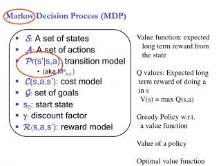
Markov Decision Process. Components: States s , beginning with initial state s 0 Actions a Each state s has actions A(s) available from it Transition model P(s’ | s, a)

Markov Decision Process
E N D
Presentation Transcript
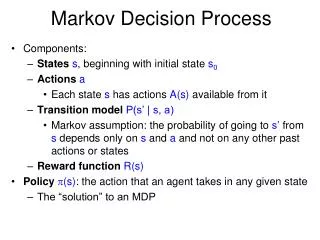
Markov Decision Process • Components: • Statess, beginning with initial state s0 • Actionsa • Each state s has actions A(s) available from it • Transition model P(s’ | s, a) • Markov assumption: the probability of going to s’ from s depends only on sand a and not on any other past actions or states • Reward functionR(s) • Policy(s): the action that an agent takes in any given state • The “solution” to an MDP
Overview • First, we will look at how to “solve” MDPs, or find the optimal policy when the transition model and the reward function are known • Next time, we will consider reinforcement learning, where we don’t know the rules of the environment or the consequences of our actions
Example 1: Game show • A series of questions with increasing level of difficulty and increasing payoff • Decision: at each step, take your earnings and quit, or go for the next question • If you answer wrong, you lose everything $100 question $1,000 question $10,000 question $50,000 question Correct: $61,100 Q1 Q2 Q3 Q4 Correct Correct Correct Incorrect: $0 Incorrect: $0 Incorrect: $0 Incorrect: $0 Quit: $100 Quit: $1,100 Quit: $11,100
Example 1: Game show • Consider $50,000 question • Probability of guessing correctly: 1/10 • Quit or go for the question? • What is the expected payoff for continuing? 0.1 * 61,100 + 0.9 * 0 = 6,110 • What is the optimal decision? $100 question $1,000 question $10,000 question $50,000 question Correct: $61,100 Q1 Q2 Q3 Q4 Correct Correct Correct Incorrect: $0 Incorrect: $0 Incorrect: $0 Incorrect: $0 Quit: $100 Quit: $1,100 Quit: $11,100
Example 1: Game show • What should we do in Q3? • Payoff for quitting: $1,100 • Payoff for continuing: 0.5 * $11,100 = $5,550 • What about Q2? • $100 for quitting vs. $4162 for continuing • What about Q1? U = $3,746 U = $4,162 U = $5,550 U = $11,100 $100 question $1,000 question $10,000 question $50,000 question 1/10 9/10 3/4 1/2 Correct: $61,100 Q1 Q2 Q3 Q4 Correct Correct Correct Incorrect: $0 Incorrect: $0 Incorrect: $0 Incorrect: $0 Quit: $100 Quit: $1,100 Quit: $11,100
Example 2: Grid world Transition model: R(s) = -0.04 for every non-terminal state
Example 2: Grid world Optimal policy when R(s) = -0.04 for every non-terminal state
Example 2: Grid world • Optimal policies for other values of R(s):
Markov Decision Process • Components: • Statess • Actionsa • Each state s has actions A(s) available from it • Transition model P(s’ | s, a) • Markov assumption: the probability of going to s’ from s depends only on s and a, and not on any other past actions and states • Reward functionR(s) • The solution: • Policy(s): mapping from states to actions
Partially observable Markov decision processes (POMDPs) • Like MDPs, only state is not directly observable • States s • Actions a • Transition model P(s’ | s, a) • Reward function R(s) • Observation model P(e | s) • We will only deal with fully observable MDPs • Key question: given the definition of an MDP, how to compute the optimal policy?
Maximizing expected utility • The optimal policy should maximize the expected utility over all possible state sequences produced by following that policy: • How to define the utility of a state sequence? • Sum of rewards of individual states • Problem: infinite state sequences
Utilities of state sequences • Normally, we would define the utility of a state sequence as the sum of the rewards of the individual states • Problem: infinite state sequences • Solution: discount the individual state rewards by a factor between 0 and 1: • Sooner rewards count more than later rewards • Makes sure the total utility stays bounded • Helps algorithms converge
Utilities of states • Expected utility obtained by policy starting in state s: • The “true” utility of a state, denoted U(s), is the expected sum of discounted rewards if the agent executes an optimal policy starting in state s • Reminiscent of minimax values of states…
Finding the utilities of states Max node • What is the expected utility of taking action a in state s? • How do we choose the optimal action? Chance node P(s’ | s, a) U(s’) • What is the recursive expression for U(s) in terms of the utilities of its successor states?
The Bellman equation • Recursive relationship between the utilities of successive states: Receive reward R(s) Choose optimal action a End up here with P(s’ | s, a) Get utility U(s’) (discounted by )
The Bellman equation • Recursive relationship between the utilities of successive states: • For N states, we get N equations in N unknowns • Solving them solves the MDP • We could try to solve them through expectimax search, but that would run into trouble with infinite sequences • Instead, we solve them algebraically • Two methods: value iteration and policy iteration
Method 1: Value iteration • Start out with every U(s) = 0 • Iterate until convergence • During the ith iteration, update the utility of each state according to this rule: • In the limit of infinitely many iterations, guaranteed to find the correct utility values • In practice, don’t need an infinite number of iterations…
Value iteration • What effect does the update have?
Method 2: Policy iteration • Start with some initial policy 0 and alternate between the following steps: • Policy evaluation: calculate Ui(s) for every state s • Policy improvement: calculate a new policy i+1 based on the updated utilities
Policy evaluation • Given a fixed policy , calculate U(s) for every state s • The Bellman equation for the optimal policy: • How does it need to change if our policy is fixed? • Can solve a linear system to get all the utilities! • Alternatively, can apply the following update: