Download

1 / 20
200 likes | 253 Views
Learn about Markov Decision Processes (MDP) in grid environments with rewards, actions, and transition models. Understand optimal policies and utilities in deterministic and stochastic processes. Explore finite and infinite horizon decision epochs.

E N D
Markov Decision Process(MDP) Ruti Glick Bar-Ilan university
+1 -1 START example • Agent is situate in 4x3 environment • Each step have to choose action • Possible actions: Up, Down, Left, Right • Terminates when reaching goal state • might be more than one goal state • Each goal state have weight • Full observable • Agent always know where it is
+1 -1 +1 -1 START START Example (cont.) • In deterministic environment solution easy: • [Up, Up, Right, Right, Right] • [Right, Right, Up, Up, Right]
0.8 0.1 0.1 Example (cont.) • But… Action are unreliable • intended effect achieved only with probability 0.8 • Probability of 0.1 getting right • Probability of 0.1 getting left • If bumps into wall – stays in place
+1 -1 +1 -1 START START Example (cont.) • by executing the sequence [Up, Up, Right, Right, Right]: • Chance of following the desired path:0.8*0.8*0.8* 0.8*0.8 = 0.85 =0.32768 • Chance of accidentally get to goal from the other path:0.1*0.1*0.1* 0.1*0.8 = 0.14 * 0.81 =0.00008 • Total of only 0.32776 to get to desired goal
Transition Model • Specification of outcome probabilities of each action in each possible state • T(s, a, s’) = Probability of reaching s’ if action a is done in state s • Can be described as 3 dimensional table • Markov assumption:The next state’s conditional probability depends only on its immediately previous state
Reward • Positive of negative reward that agent receives in state s • Sometimes reward is associated only with state • R(S) • Sometimes reward is assumed associated with state and action • R(S, A) • Sometimes, reward associated with state, action and destination-state • R(S,A,J) • In our example: • R([4,3]) = +1 • R([4,2]) = -1 • R(s) = -0.04, s ≠ [4,3] and s ≠ [4,2] • Can be seen as the desired of agent staying in game
Environment history • Decision problem is sequential • Utility function depend on sequence of state • Utility function is sum of rewards received • In our example: • If reached (4,3) after 10 steps than total utility= 1+10*(-0.04) = 0.6
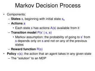
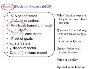
Markov Decision Process (MDP) • The specification of a sequential decision problem for a fully observable environment that satisfies the Markov Assumption and yields additive rewards. • Defined as a tuple: <S, A, P, R> • S: State • A: Action • P: Transition function • Table P(s’| s, a), prob of s’ given action a in state s • R: Reward • R(s) = cost or reward being in state s
In our example… • S: State of the agent on the grid • E.g. (4,3) • Note that cell denoted by (x,y) • A: Actions of the agent • i.e. Up, Down, Left, Right • P: Transition function • Table P(s’| s, a), prob of s’ given action “a” in state “s” • E.g., P( (4,3) | (3,3), Up) = 0.1 • E.g., P((3, 2) | (3,3), Up) = 0.8 • R: Reward • R(3, 3) = -0.04 • R (4, 3) = +1
Solution to MDP • In deterministic processes, solution is a plan. • In observable stochastic processes, solution is a policy • Policy: a mapping from S to A • A policy’s quality is measured by its EU Notation: π ≡ a policy π(s) ≡ the recommended action in state s π* ≡ the optimal policy (maximum expected utility)
Following a Policy Procedure: 1. Determine current state s 2. Execute action π(s) 3. Repeat 1-2
Optimal policy for our example The reward is small relative to -1. prefer to go around then falling into -1. +1 -1 R(4,3) = +1 R(4,2) = -1 R(S) = -0.04 START
Optimal Policies in our example +1 +1 -1 -1 START START R(Start) < -1.6284 -0.4278 < R(Start) < -1.6284 Life so painful – the agent run to the nearest exit Life unpleasant – the agent trying to get +1, willing to to risk and fall into -1
Optimal Policies in our example +1 +1 -1 -1 START START -0.0221 < R(S) < 0 R(s) > 0 Life is nice – the agent takes no risks at all Agent wants to stay at game
Decision Epoch • Finite horizon • After fixed time N the game is over. Nothing matters. • Uh([s0, s1, …, sN+k]) = Uh([s0, s1, …, sN]), for all k>0 • Optimal action might change over time • Infinite horizon • no fixed deadline • No reason to behave differently in same state at different time • We will discuss this case
example +1 • If agent in (1,3). what will it do? • In Finite horizon where N=3 will go up • In Infinite horizon – depend on other parameters -1 Agent here
Assigning Utility to Sequences • Additive reward • Uh([s0, s1, s2, …]) = R(s0) + R(s1) + R(s2) + … • In our last example we used this method • Discounted Factor • Uh([s0, s1, s2, …]) = R(s0) + γR(s1) + γ2R(s2) + … • 0 < γ < 1 • γrepresent the chance the world will continue exist • We will assume discounter reward
additive reward • Problem • For infinite horizon if the agent never get to terminate state, the utility will be infinite. Can’t compare between +∞ and +∞ • Solutions • With discount reward the utility of infinite sequence is finiteUh([s0, s1, s2, …]) = • Proper policy = policy that guaranteed to get to finite state • Compare infinite sequences in term of average reward
conclusion • Discount reward is the best solution for infinite horizon • Policy πrepresent a group of possible sequences • Specific probability of each case • Value of policy is the expected sum of all possible state sequences