Download
1 / 23
230 likes | 385 Views
Pole balancing robot and some control strategies. | x. f . θ. Introduction. A sketch of PBR (Pole Balancing Robot). Figure1: Pole balancing Robot. Robotic vehicle would operate on the top of the table provided (refer to Fig.2a). Fig.2.a. Pole Balancing Robot Table.

E N D
| x f θ Introduction • A sketch of PBR (Pole Balancing Robot) Figure1: Pole balancing Robot
Robotic vehicle would operate on the top of the table provided (refer to Fig.2a). Fig.2.a. Pole Balancing Robot Table • Tabletop will have a slight gradient at the start (region A) and the end (region C) <shown in Fig.2a>
A metallic wedge of cross section shown in Fig.2b.(not to scale) will be used as an obstacle. • The length of the wedge will match the width of the table. • The wedge will be painted to match the table surface. • A retro-reflective tape will be stuck to it at the middle to match the one on the table. • The judge will place the wedge in region B any where between the inner edges of the two innermost tapes so that the wedge is perpendicular to the path. • It will not be moved thereafter.
Vehicle will be placed within the region A (See Fig. 2b). Fig.2.b Wedge Section (Enlarged View) • The operator may move the inverted pendulum to an upright position and release it upon receiving the signal from the judges. • The vehicle must balance the pole in the upright position for a minimum of 20 seconds without the vertical pole crossing the line X-X'.
Upon completion of the task above, • vehicle should move across the line X-X' once • move through the region B, until the pole clears the line Y-Y', without losing balance during transit not hitting any part of the table or its own chassis • Upon completion of the task above, • vehicle must retrace the path, cross the line X-X' again and get back to region A. This will complete one cycle. • This time, during the retrace, the vehicle need not stay any length of time at region B or A, before the start of the second cycle.
When an electronic sensing system is used for detecting the pole crossing Y-Y’ and X-X’ lines, the pole sensors at both sides will be placed such that the line of sight of the sensors will be 20 cm above the lines marked on the platform. • This may warrant that the robot moves further for the pole to intercept the line of sight of the sensors. • This is important since many robots have their poles inclined inwards towards the centre of platform at these points of turning back.
Furthermore, no part of the robot other than the pole should be above 15 cm so that no other part of the robot (except the pole) would trigger the sensor. • The vehicle should repeat these cycles. • To count these cycles as successful cycles they must be followed by at least 20 seconds of static balancing at region A. • The robot may continue on (untouched) for more cycles, and complete them with 20 seconds of static balancing at the end, which if successful will be counted cumulatively. • If a robot is touched by the handler during the trial, it must be restarted for the next attempt.
1 2 Pole Balancing Robot Dynamics • The line diagram of a pole balancing robot is shown in Fig.1. • The following equations can be written to describe the dynamics of the robot movement and the pole angle,θ. [(M+m)s2 + Bs] X(s) + [(ml)s2 + (b/l)s] (s) = F(s) ms2 X(s) + [mls2 + (b/l)s - mg] (s) = 0
3 • One Possible Approach: where, M = mass of the vehicle B = linear equivalent friction of the vehicle m = mass of the pole b = rotational friction of the pole g = 9.81 m/s2 l = half length of the pole x = distance = angle in radians
4 5 -mS mls2 + (b/l).S - mg (s) V(s) V(s) = s.X(s) • We can move a S from RHS to denominator. Hence, • But, • The above Eqn.5 can be represented by Fig.3. Figure.3. Angle versus velocity
7 8 F(s) V(s) 1 M s + B • a mass, M and • friction coefficient, B, • we can draw, • for a given force f, • Getting back to the problem at hand, for any vehicle with Fig 4.Force acting on a vehicle • But torque is written as, • Also torque can be written as,
9 10.a • Where r = diameter of the driving wheel §§ It has been assumed that there is only one motor §§ • However, defining back emf as Eb, Eb = Kb.m Where, mis the motor’s rotational velocity.
10.b 10.c But, Where, w is the driving wheel’s rotational velocity v = r.w
Kt.Ng ---------- Ra r 1 ---------- MS+B 11 Kb.Ng -------------- r Vs V • Connecting the above equations, a block diagram can be drawn Figure.5.Block diagram relating applied voltage to velocity This can be simplified as:
With the above system as the core plant , one can produce a velocity control block diagram. Figure 6.Velocity Control of robotic vehicle Where Tpwm = PWM Period [half period] del = ‘ON’ fraction G = Numerical Gain
Block diagram can be drawn. Figure 7.Complete Block Diagrams • It all looks very complicated. • Note that it is still first order dynamics.
V(s) VR(s) Gm Mm.S + Bm Figure 8.Simplified Dynamics • Once you get the numbers, it is not as complicated as it appears. Numerical Example: Let G = 1000 Tpwm = 1000 Kt = 0.033 Ng = 8.0 (gear ratio) r= 3 cm M = 2.5 Kg Ra = 6 B = 2 Kb = Kt Vs = 28 Volts Then the parameters can be easily computed.
(S) V(S) VR -mS mls2 + (b/l).S - mg Gm Mm.S + Bm • To get the overall picture, let us combine Fig 3 and Fig.8 Figure 9. Angle Versus Velocity Dynamics of a Pole balancing robot
Control Options: • Common Strategy: • Since there two outputs but only one manipulated variable. • In all our design we use two loop system. • The position reference is in the outer loop and the error generated is used as the angle reference to the inner loop to keep the pole vertical. • Actually many variations are possible.
Implementation can be done using one of the following techniques: • Polynomial based controllers: In this controllers, one can describe the transfer function and form z-domain system and use a pole placement or LQC algorithms to derive a controllers. At times LQC controller may go unstable. • State space controllers: One can take a state apace model with x, v, angle, angular velocity as states. Again pole placement controllers can be implemented. • PD Controller: Simple proportional and derivative controllers also would work. But such system is only conditionally stable.
Typical PBR • In our design, • use eZdsp™ mother board • robot uses potentiometer, and one drop encoder. • drivers are H-bridge drivers controlling two motors. Fig.9. Typical PBR
CONCLUSION During this brief talk, • The basic competition event was described • The model of a pole balancing robot as a single input, multi-output system was derived • Possibility of a two loop controller structure was discussed • A few controller design options were suggested.