Download
1 / 23
230 likes | 253 Views
Explanation of simple linear regression model, equations, estimation of coefficients, interpretation of results, and assessing model goodness.

E N D
A scatter plot gives a compact illustration of the distribution of two variables and the association / correlation between the variables • When there is causation/ or hypothesize causation,we want to find the relatioship between the two variables.
Given two variables ,say X ( height )and • Y( weight ) and if X is the cause leading to changes in Y ( effect ) , then our interest will be to determine a mathematical relationship ( model ) between X and Y and use it to predict Y for given X. • Here X is called independent variable and Y is called dependent variable.
Regression analysis is a statistical procedure used to find relationships among a set of variables • In simple linear regression ,we find linear relationship between one independent ( X ) and one dependent variable ( Y ). • The model is called simple linear regression model .
The values of the independent variable are fixed and measured without error/ negligible error ( this is not a rigid assumption; the values need not be fixed in the sense they are nonrandom. They could be the values realised by a random variable also ) • For each value of X there is a subpopulation of Y values
For the validity of statistical inference, this subpopulation is normally distributed with equal variances • The means of all the subpopulations fall on the same straight line. This is the assumption of linearity • The Y values are statistically independent
Based on these assumptions we formulate the following statistical model,called the simple linear regression model: • y = α +β x + e • Here ‘y’ is a typical value from one of the subpopulations of Y, α and β are the regression coefficients and e is called the error term. • The error term is normally distributed
Given sample data on X and Y, we try to estimate the parameters( regression coefficients) in the model and construct the sample regression equation. The sample regression equation is a linear equation, such as: y = a + bx Where ‘a’ and ‘b’ are the estimates of α and β
y = a + bx • y is the dependent variable • x is the independent variable • a is a constant ( called intercept ) • b is the slope of the line • For every increase of one unit in x, y changes by an amount equal to b • Some relationships are perfectly linear and fit this equation exactly.
Estimating the regression coefficifients • Using a sample of n pairs of (x , y ) values, the coefficients ‘a’ and ‘b’ are given by the following formulas:
After getting ‘b’ ‘a’ can be determined from the following formula: • Where and are the sample means of x and y respectively.
Weight, for instance, is to some degree a function of height, but there are variations that height does not explain. On average, you might have an equation like: Weight = -222 + 5.7*Height If you take a sample of actual heights and weights, you might see something like the graph to the right.
The line in the graph shows the average relationship described by the equation. Often, none of the actual observations lie on the line. The difference between the line and any individual observation is the error. The new equation is: Weight = -222 + 5.7*Height + e This equation does not mean that people who are short enough will have a negative weight. The observations that contributed to this analysis were all for heights between 5’ and 6’4”. The model will likely provide a reasonable estimate for anyone in this height range. You cannot, however, extrapolate the results to heights outside of those observed. The regression results are only valid for the range of actual observations.
Regression finds the line that best fits the observations. It does this by finding the line that results in the lowest sum of squared errors. This principle is called the Principle of Least Squares. Since the line describes the mean of the effects of the independent variables, by definition, the sum of the actual errors will be zero. If you add up all of the values of the dependent variable and you add up all the values predicted by the model, the sum is the same. That is, the sum of the negative errors (for points below the line) will exactly offset the sum of the positive errors (for points above the line). Summing just the errors wouldn’t be useful because the sum is always zero. So, instead, regression uses the sum of the squares of the errors
How Good is the Model? One of the measures of how well the model explains the data is the R2 value. Differences between observations that are not explained by the model remain in the error term. The R2 value tells you what percent of those differences is explained by the model. An R2 of .68 means that 68% of the variance in the observed values of the dependent variable is explained by the model, and 32% of those differences remains unexplained in the error term.
Regression and correlation are two powerful statistical tools when properly used.incorrect usage can lead to meaningless results. Here are some precautionary notes. • Go through the assumptions underlying correlation and regression before collecting data. It may be difficult to assess all the assumptions and the gap existing between the assumptions and the data. First judge the adequacy of the approach and when you are confident,use it for analysing your data.
Computation of R-square • The following sum-of –squares(SS) are defined: • Where is the predicted value of y and
A significant correlation between two variables,say X and Y may mean one of several things below; • X causes Y • Y causes X • Effect of large sample giving high correlation while,in fact, X and Y are not correlated. • Some third factor ,directly or indirectly induces correlation between X and Y
Identify the model – decide whether only correlation analysis is relevant or regression analysis has to be carried out. • Review the assumptions since validity of the conclusions depend on the choice of the model and the validity of the model assumptions • If regression analysis is carried out, validate the model using proper diagnostic checks, such as value,ANOVA ( for testing the significance of and testing for significance of the regression coefficients). If the model is to be used for prediction purpose, it is better to validate the model with an independent sample.Do not use the model to predict Y for values of X beyond its range of values.
After validating the model,it can be used for • Predicting the value of Y for a given value of X • To estimate the mean of a subpopulation of Y for a given value of X
Peat & Barton: Medical Statistics - A Guide to Data Analysis, Blackwell/BMJ Publishers • Harris & Taylor : Medical Statistics Made Easy, Martin Dunitz Publishers • Dunn & Clark : Basic Statistics – A Primer for the Biomedical Sciences