Chandy-Lamport Algorithm for Termination and Deadlock Detection in Distributed Systems
250 likes | 377 Views
This document discusses the Chandy-Lamport algorithm for detecting termination and deadlocks in distributed computing environments. It elaborates on process interactions, broadcast mechanisms, and global state consistency. The text explores the implications of communication topology, specifically strongly connected graphs, in ensuring reliable state collection. Additionally, it addresses deadlock principles such as resource exclusivity and circular waiting, presenting techniques for detection, prevention, and recovery, including Dijkstra-Scholten's algorithm and the concept of distributed deadlock.

Chandy-Lamport Algorithm for Termination and Deadlock Detection in Distributed Systems
E N D
Presentation Transcript
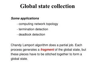
Global state collection Some applications - computing network topology - termination detection - deadlock detection Chandy-Lamport algorithm does a partial job. Each process generates a fragment of the global state, but these pieces have to be “stitched together” to form a global state.
Once the pieces of a consistent global state become available, consider collecting the global state via all-to-all broadcast At the end, each process will compute a set V, where V= {s(i): 0 ≤ i ≤ N-1 } A simple exercise s(i) s(j) i j s(k) s(l) k l
All-to-all broadcast Assume that the topology is a strongly connected graph V.i W.i V.k W.k (i,k) (j,i) V.j W.j Acts like a “pump”
Lemma. empty (i, k) ⇒W.i ⊆ V.k. Use a simple inductive argument. (Upon termination) ∀i: V.i = W.i, and all channels are empty. So, V.i ⊆ V.k. In a strongly connected graph, every node is in a cycle On a cyclic path, V.i = V.k must be true. Since s(i)∈V.i, s(i)∈V.k. Proof outline V.i W.i V.k W.k (i,k) i k
Lemma. The algorithm will terminate in a bounded number of steps. Consider the variant function Proof outline V.i W.i V.k W.k Channel states (i,k) i k Statement 1 and Statement 2 increase Y lexicographically, until the V’s reach their largest value {s(0), s(1), s(2), …, s(n-1)}. So the algorithm terminates in a bounded number of steps.
Termination detection During the progress of a distributed computation, processes may periodically turn active or passive. A distributed computation termination when: (a) every process is passive, (b) all channels are empty, and (c) the global state satisfies the desired postcondition
Visualizing diffusing computation initiator active passive Notice how one process engages another process. Eventually all processes turn white, and no message is in transit -- this signals termination. How to develop a signaling mechanism to detect termination?
An initiator initiates termination detection by sending signals (messages) down the edges via which it engages other nodes. At a “suitable time,” the recipient sends an ack back. When the initiator receives ack from every node that it engaged, it detects termination. Node j engages node k. Dijkstra-Scholten algorithm The basic scheme j k signal j k j k ack
Deficit (e) = # of signals on edge e - # of ack on edge e For any node, C = total deficit along incoming edges and D = total deficit along outgoing edges edges For the initiator, by definition, C = 0 Dijkstra-Scholten algorithm used the following two invariants to develop their algorithm: Invariant 1. (C ≥ 0) ⋀ (D ≥ 0) Invariant 2. (C > 0) ⋁ (D = 0) Dijkstra-Scholten algorithm 0 1 2 3 4 5
The invariants must hold when an interim node sends an ack. So, acks will be sent when (C-1 ≥ 0) ⋀ (C-1 > 0 ⋁ D=0) {follows from INV1 and INV2} = (C > 1) ⋁ (C ≥1 ⋀ D=0) = (C > 1) ⋁ (C =1 ⋀ D=0) Dijkstra-Scholten algorithm 0 1 2 3 4 5
program detect {for an internal node i} initially C=0, D=0, parent = i dom = signal ⋀ (C=0) → C:=1; state:= active; parent := sender {Send signals to engage other nodes, or turn passive} [] m = ack → D:= D-1 [] (C=1⋀ D=0) ⋀ state = passive → send ack to parent; C:= 0; parent := i [] m = signal ⋀ (C=1)→ send ackto the sender; od Dijkstra-Scholten algorithm 0 1 2 3 4 5 Note that the parent relation induces a spanning tree
Distributed deadlock When each process waits for some other process (to do something), a deadlock occurs. Assume each process owns a few resources. Review how resources are allocated, and how a deadlock is created. Three criteria for the occurrence of deadlock - Exclusive use of resources - Non-preemptive scheduling - Circular waiting by all (or a subset of) processes
Distributed deadlock Three aspects of deadlock • deadlockdetection • deadlock prevention • deadlock recovery
Distributed deadlock • May occur due to bad designs/bad strategy [Sometimes prevention is more expensive than detection and recovery. So designs may not care about deadlocks, particularly if it is rare.] • Caused by failures or perturbations in the system
Distributed Deadlock Prevention uses pessimistic strategies An example from banker’s problem (Dijkstra) A banker has $10,000. She approves a credit line of $6,000 to each of the three customers A, B, C. since the requirement of each is less than the available funds. • The customers can pay back any portion of their loans at any time. Note that no one is required to pay any part of the loan unless (s)he has borrowed up to the entire credit line. • However, after the customer has borrowed up to the entire credit line ($6000) (s)he must return the entire money is a finite time. • Now, assume that A, B, C borrowed $3000 each. The state is unsafe since there is a “potential for deadlock.” Why?
Banker’s Problem Questions for the banker Let the current allocations be A = $2000, B = $2400, $C=$1800. 1. Now, if A asks for an additional $1500, then will the banker give the money immediately? 2. Instead, if B asks for $1500 then will the banker give the money immediately?
Represents who waits for whom. No single process can see the WFG. Review how the WFG is formed. Wait-for Graph (WFG) p1 p0 p3 p2 p4
Resource deadlock [R1 AND R2 AND R3 …] also known as AND deadlock Communication deadlock [R1 OR R2 OR R3 …] also known as OR deadlock Another classification p0 p1 p3 p2 p4
Notations w(j) = true ⇒ (j is waiting) depend [j,i] = true⇒j ∈ succn(i) (n>0) (i’s progress depends on j’s progress) P(i,s,k) is a probe (i=initiator, s= sender, r=receiver) Detection of resource deadlock 2 1 3 4 P(4, 4, 3) initiator
{Program for process k} do P(i,s,k) received ⋀ w[k] ⋀ (k ≠ i) ⋀¬ depend[k, i] → send P(i,k,j) to each successor j; depend[k, i]:= true [] P(i,s,k) received ⋀ w[k] ⋀ (k = i) →process k is deadlocked od Detection of resource deadlock
To detect deadlock, the initiator must be in a cycle Message complexity = O(|E|) (edge-chasing algorithm) Observations E=set of edges of the WFG
Communication deadlock 5 This WFG has a resource deadlock but no communication deadlock
A correction The definition of knot in page 147 is not correct. The correct definition is: A knot in a directed graph is a subgraph induced by a set of vertices with the property that (1) every vertex in the knot has at least outgoing edge, and (2) all outgoing edges from the vertices in the knot connect to other vertices in the knot. Thus it is impossible to leave the knot while following the directions of the edges.
A process ignores a probe, if it is not waiting for any process. Otherwise, first probe→ mark the sender as parent; forwards the probe to successors Not the first probe→ Send ack to that sender ack received from every successor→ send ack to the parent Communication deadlock is detected if the initiator receives ack. Detection of communication deadlock Has many similarities with Dijkstra-Scholten’s termination detection algorithm