Download
1 / 1
10 likes | 126 Views
MAP Estimation of Semi-Metric MRFs via Hierarchical Graph Cuts. M. Pawan Kumar Daphne Koller. MAP Estimation. b ( k). Semi-Metric Potentials. Bounds.

E N D
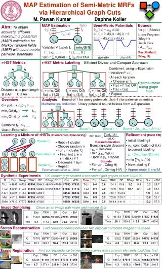
MAP Estimation of Semi-Metric MRFs via Hierarchical Graph Cuts M. Pawan Kumar Daphne Koller MAP Estimation b(k) Semi-Metric Potentials Bounds Aim:To obtain accurate, efficient maximum a posteriori (MAP) estimation for Markov random fields (MRF) with semi-metric pairwise potentials lk a(i) ab(i,k) = wab d(i,k) For =1 (Metric) li ab(i,k) d(i,i) = 0, d(i,j) = d(j,i) > 0 Linear Program: O(log H) va vb d(i,j) - d(j,k) ≤ d(i,k) Graph Cuts: 2 dmax/dmin minf Q(f) Variables V, Labels L f : {a,b, …} {1, …, H} Our Method: O(log H) Q(f) = ∑ a(f(a)) + ∑ ab(f(a),f(b)) f(a)-f(b) f(a)-f(b) r-HST Metrics r-HST Metric Labeling Efficient Divide-and-Conquer Approach Combine fi using -Expansion A A • Initialize f0 = f1 • At each iteration • Choose an fi • ft(a) = ft-1(a) OR • ft(a) = fi(a) B B C C Optimal move using graph cuts l1 l2 l3 l4 l1 l2 l3 l4 l5 l6 Distance dT path length f1 = minf Q(f) f2 = minf Q(f) f3 = minf Q(f) • Repeat C ≤ A/r B ≤ A/r f(a) {1,2} f(a) {3,4} f(a) {5,6} Analysis Overview Bound of 1 for unary potentials, 2r/(r-1) for pairwise potentials Mathematical Induction Unary potential bound follows from -Expansion d 1dT1 + 2dT2 + …. A A minfQ(f;dT1) fT1 minfQ(f;dT2) fT2 B B . C C . va vb va vb va vb l1 l2 l3 l4 Combine fT1, fT2 …. Bound = 2dmax/dmin = 2r/(r-1) Bound = 1 Bound = 1 True for children Use -Expansion Learning a Mixture of rHSTs (Hierarchical Clustering) Refinement (Hard EM) ∑tdTt(i,k) min maxi,k d(i,k) • Initial labeling f l1 l3 l4 Cluster Cj Derandomization • Root 1 cluster Boosting-style descent • yik: contribution of (i,k) • to current labeling • Choose random π • yik = Residual • For li in cluster Cj • Find first lk in π • s.t. d(i,k) ≤ T • min ∑yik dT(i,k) l2 l3 l1 l4 Permutation π yik = ∑wab[f(a)=i][f(b)=k] • Update yik. Repeat. • min ∑yik dT(i,k) l3 Bounds • Decrease T by r • New labeling f’ • For =1, O(log H) Cluster Cj+1 • Repeat l4 l1 • For 1, O((log H)2) • Approximate E and M Fakcharoenphol et al., 2000 Synthetic Experiments 100 randomly generated 4-connected grid graphs of size 100x100 Image Denoising Clean up an image with noise and missing data Stereo Reconstruction Find correspondence between two epipolar corrected images of a scene Scene Registration Find correspondence between two scenes with common elements (building, fire)