Download
1 / 54
540 likes | 656 Views
Statistics Review II. Types of statistical analyses (and when you use them) one sample z test one sample t test independent samples t test paired samples t test Pearson correlation one-way chi square one-way b/w subjects ANOVA one-way w/in subjects ANOVA multi-factor ANOVA w/in subs

E N D
Types of statistical analyses (and when you use them) one sample z test one sample t test independent samples t test paired samples t test Pearson correlation one-way chi square one-way b/w subjects ANOVA one-way w/in subjects ANOVA multi-factor ANOVA w/in subs b/w subs mixed multiple regression
Types of statistical analyses (and when you use them) one sample z test - you know population mean and s.d. - test if sample mean differs from population mean example: you want to determine if the mean IQ of adopted children differs from the general population of children 1. H0: m = 100 2. set a to .05 3. n = 25, X = 96 4. SEM = 15/5 = 3 5. compute p that a X of 96 would be observed in a sampling dist. where m = 100, and SEM = 3
Two-Tail Test • we want to know if the IQ of the adopted kids is different from the pop. • We don’t care if the adopted kids are smarter or dumber than the pop. • We use a two-tailed test
Choosing Your Criterion (alpha) • Alpha (a) is the p that you select as the cut-off point for rejecting the null hypothesis.
2.5% 2.5% m = 100 Choosing Your Criterion rejection region
Region of Rejection • If you have a two-tailed test and you set the alpha to be 0.05 • This means that you want to see if your sample falls in either the highest 2.5% or the lowest 2.5% of the distribution…reject H0 • What z score would you need on either side to reject the Ho?
Determine Your Critical z score • We want to look up the z-scores in which .025 of the curve is beyond the z score • zcrit = +/- 1.96 2.5% 2.5% -1.96 m = 100 +1.96
Sample z-score • You need to calculate z and compare it to zcrit • We call this zobtained (zobt) zobt = X – m sC
What if zobt < zcrit ? • we fail to reject Ho • The sample mean is different than the population mean by chance. • We call this a nonsignificant result. • means that we think that our sample mean is from the sampling distribution determined by CLT under the null hypothesis.
What if zobt > zcrit ? • Significant: this means that we have rejected Ho and have accepted Ha • These results are unlikely to occur if the null hypothesis is correct • Therefore, we conclude that the null hypothesis is not correct
Calculate zobt for adopted kids when X = 96 zobt = X – m sC First, calculate the sC = sC N • sC = 15 = 15 = 3 zobt = X – m = 96 - 100 • 25 5 sC 3.0
Look at that z z = 96 – 100 = -1.33 3.0 So, what does this mean? Compare to the zcrit of +1.96 We conclude that difference b/w sample mean and population mean is not sig., i.e. the difference is due to sampling error
Determine Your Critical z score • We want to look up the z-scores in which .025 of the curve is beyond the z score • zcrit = +/- 1.96 2.5% 2.5% m = 100 -1.96 -1.33
What if zobt > zcrit ? • Let’s say our mean was 94 instead of 96. zobt. = X – m = 94 -100 = -6 = - 2.0 sC 3 3
Determine Your Critical z score • We want to look up the z-scores in which .025 of the curve is beyond the z score • zcrit = +/- 1.96 2.5% 2.5% m = 100 -2.0 -1.96
Types of statistical analyses (and when you use them) one sample t test – the same as the z test except that SEM is estimated by s example: you want to determine if a particular diet is successful. 10 overweight people diet for 1 month and lose an average of 3.11 lbs. (mean = 3.11, s = 5.62) 1. H0: m = 0 2. set a to .05 3. n = 10, X = 3.11 4. SEM = 5.62/3.16 = 1.78 5. compute p that a X of 3.11 would be observed in a sampling dist. where m = 0, and SEM = 3
Look at that t t = 3.11 – 0 = 1.75 1.78 So, what does this mean?
Prediction • those on the diet will lose weight • One-tailed test –use when you predict the direction in which scores will change. 1.75 0 1.83 amount of weight lost
Look at that t t = 3.11 – 0 = 1.75 1.78 So, what does this mean? Compare to the tcrit of 1.83 We conclude that difference b/w sample mean and population mean is not sig., i.e. the difference is due to sampling error
Experimental Designs Within Subjects Between Subjects
Types of statistical analyses (and when you use them) independent samples t test example: you want to see if milk chocolate improves quiz scores. Ten students are given 13.7 grams of milk chocolate at study and test, and 9 students are given 16 grams of caramel at study and test. Xchoc = 85.0 Xcarm = 77.8 H0: mchoc - mcarm< 0 t (17) = .976, p > .34 ways to increase power - increase N - make IV more extreme - make DV more sensitive .976 1.74 t values under null hypothesis We conclude that difference b/w means is not sig., i.e. the difference is due to sampling error
Types of statistical analyses (and when you use them) paired samples t test example: Wechsler examined the practice effect in a preschool IQ test. Fifty 5-year old children were tested, then retested 2-4 months later. Xt1 = 105.6 Xt2 = 109.2 r = .91 t (49) = 4.16, p < .05 4.16
Types of statistical analyses (and when you use them) Pearson correlation example: test to see if there is a relationship b/w GRE verbal scores and final exam scores in stats (N = 20). H0: r = 0 r (18) = .543, p < .05 r = .543 r = 0 r =.44
Types of statistical analyses (and when you use them) one-way chi square example: in a wine tasting test, 50 participants taste an ounce of German wine and an ounce of French wine. They choose the one that they prefer.
Measurement Scales nominal data are categorical Type of wine preferred Expected value - null German 20 25 French 30 25 c2 (1) = 2.0, p > .15
Measurement Scales nominal data are categorical Type of wine preferred Expected value - null German 18 25 French 32 25 c2 (1) = 3.92, p < .05
Background Information False Memory and Memory Reconstruction Loftus and Palmer (1974) Participants witness a film of a car accident. Participants divided into 3 groups: About how fast were the cars going when they _____ each other? 1. hit 2. smashed into 3. control group - not asked any questions
Leading Questions and Memory Distortion Loftus & Palmer (1974) participants viewed car accident About how fast were the cars going when they _____ each other? Group 1 - hit (34 mph) Group 2 - smashed into (41 mph) Group 3 - control group - no questions Memory reconstruction or response bias? est. speed hit smashed
Leading Questions and Memory Distortion Loftus & Palmer (1974) participants viewed car accident proportion reporting broken glass control hit smashed
Types of statistical analyses (and when you use them) one-way b/w subjects ANOVA example: 150 students are randomly assigned to three classes, 50 students per class. The same instructor is used for all 3 classes, but a different text is used in each one. All students take the same test at the end of the course. Do the scores differ significantly across classes? (The treatment is textbook.)
1 = error variance 2 = treatment variance 3 = total variance
F Distribution H0: m1 = m2 = m3 Expected value under the null hypothesis is 1
Types of statistical analyses (and when you use them) one-way w/in subjects ANOVA example: 36 participants receive 3 types of lists in the DRM paradigm (semantic, phonological, hybrid), and the prop. of false recall is measured. F (2, 70) = 6.25, p < .05
Experimental Designs Factorial Design – 2 Independent Variables Within Subjects Between Subjects Mixed
Testing for Main Effects and Interactions (multi-factor ANOVA) Main Effect – Determining if one IV has an effect on the DV Interaction – Determining if the effect of one IV remains constant at each level of the other IV
Confirmation bias - interpreting new info. to be consistent with current beliefs
Confirmation Bias Darley and Gross (1983) Participants rated academic potential of Hannah DV = grade level rating IV #1 = Class Group 1 – Hannah – upper middle class Group 2 – Hannah – lower class IV #2 = Video Status Group 1 – no video Group 2 – see video
Seidenberg (1985) High Frequency Low Frequency Regular help punt Exception have pint
Seidenberg (1985) High Frequency Low Frequency Regular 541 554 Exception 541 584 Effect 0 -30
Payne (2001) Object Gun Tool Black 423 453 Race of Face White 440 445 Effect -17 8