Inferential Statistics II
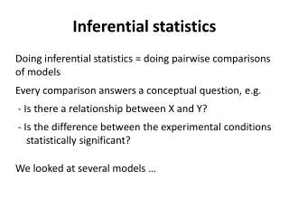
Inferential Statistics II. Confounding Variations. Anticipating the direction of the change in mean scores The similarity of the samples Random selection Sample size Multiple simultaneous t -tests. Direction. Anticipated Mean Shift. 5% (.05).

Inferential Statistics II
E N D
Presentation Transcript
Confounding Variations • Anticipating the direction of the change in mean scores • The similarity of the samples • Random selection • Sample size • Multiple simultaneous t-tests
Direction Anticipated Mean Shift 5% (.05) In some cases it can be assumed that the difference between means scores will represent a positive shift. When we give a lesson we expect that the test scores will rise from pre to post test.
Direction Anticipated Mean Shift 5% (.05) In some cases it can be assumed that the difference between means scores will represent a negative shift. If we do conflict management training we would anticipate that the number of conflicts would be reduced.
Direction ? 5% (.05) 5% (.05) What happens if you can’t anticipate which way the mean will shift? Will canceling inter-mural sports affect achievement positively or negatively?
Direction p < .05 ? 2.5% (.025) 2.5% (.025) The possible means which would be considered significant must be split to both ends of the sampling distribution—a two-tailed test of significance. It is the researchers job to demonstrate that a significance test should be one-tailed or two-tailed.
EZAnalyze always reports two-tailed results To compute one-tailed results divide p value in half.
Direction p < .05 ? 5% (.05) 5% (.05) 2.5% (.025) 2.5% (.025)
Confounding Variations • Anticipating the direction of the change in mean scores • The similarity of the samples • Random selection • Sample size • Multiple simultaneous t-tests
Similarity of Samples • Paired—Significance is easier to demonstrate if the two samples include exactly the same individuals. The random error based on the respondents being different is gone. • Independent Samples—Significance is more difficult to demonstrate if the two groups are dissimilar. Random error that appears because the respondents are different has to be accounted for.
Confounding Variations • Anticipating the direction of the change in mean scores • The similarity of the samples • Random selection • Sample size • Multiple simultaneous t-tests
Random Selection • With random sampling all members of the population to which you wish to generalize have an equal chance of being in the sample. • Scientific studies use true random sampling which is also called probability sampling. (simple and stratified) • When all of the members of a population do not have an equal chance of being in the sample it is called nonprobablity sampling. (samples of convenience) • If your sample is random you have to carefully explain how you made it that way. (methods section) • If the sample isn’t random then you have to work hard at showing that your sample is not potentially dissimilar from the population. (methods section)
Random Error • Random normal variation in groups. • Outside of the researchers control. • Inferential statistics deals with random error really well. • That is why groups should be formed randomly. • We will figure out how to deal with non-random error when we talk about validity.
Dealing with Non-Random Samples • Carefully explain how the sample was formed in the methods section. • Carefully describe important elements of the context of the study that support the idea (or not) that the sample is like the population. • Carefully explain how the analysis of data will be done. • List the possible effect of sampling procedures in the limitations section of the conclusions.
Confounding Variations • Anticipating the direction of the change in mean scores • The similarity of the samples • Random selection • Sample size • Multiple simultaneous t-tests
Sample Sizes n=1000 n=100 n=30 Population Distribution As the sample size increases the Sampling Distribution of the Mean gets narrower.The standard error gets numerically smaller.
Effect Size(Practical Significance) • With large samples it is possible that significant differences will appear from very small mean differences. • When statistical significance appears, practical significance can be reported by showing the mean differences in units of standard deviation—not standard error (remember z scores). • The simplest calculation is to determine the distance between the two mean scores and divide by the average standard deviation. (Cohen’s d) • Effect sizes over .5 are considered substantial.
Effect Size—Practical Significance How many standard deviations is the new mean from the first mean?Effect size of .2 is weak; .5 is moderate; .8 is strong
Practical SignificanceThe difference of the means in units of standard deviation T ab l e 1 M ean S c ore s on Johnson P r ob l em So lv ing I nven t or y f or S t uden t s W it h and Wit hou t Con fli c t Re s o l u t ion T ra i n i ng . Pre-Test Post-Test N = 36 N = 36 M e an 74 . 61 82 . 61* S D 13.35 11.85 = p < .0 1 * Difference in means: 74.61 - 82.61= -8 Average standard deviation: (13.35 + 11.85)/2 = 12.6 Practical significance: -8/12.6 = -.63
Practical SignificanceThe difference of the means in units of standard deviation T ab l e 1 M ean S c ore s on Johnson P r ob l em So lv ing I nven t or y f or S t uden t s W it h and Wit hou t Con fli c t Re s o l u t ion T ra i n i ng . Only report practical significance if the mean differences are statistically significant to begin with. Pre-Test Post-Test N = 36 N = 36 M e an 74 . 61 82 . 61* S D 13.35 11.85 = p < .0 1 * Difference in means: 74.61 - 82.61= -8 Average standard deviation: (13.35 + 11.85)/2 = 12.6 Practical significance: -8/12.6 = -.63
Confounding Variations • Anticipating the direction of the change in mean scores • The similarity of the samples • Random selection • Sample size • Multiple simultaneous t-tests
Research Design Groups by Treatment(Independent Variable) Data Gathering Events(Dependent Variable)
group data group data Did direct instruction improve students’ ability to recall math facts? Independent ⇓ Dependent Pre-Test Post-Test DI to 4th Grade Class t –test, paired if possible
group data group data Do students who receive DI achieve better than those that don’t? Independent ⇓ Dependent Test DI to 4th Grade Class Non-DI to different 4th Grade Class t –test, independent samples
group data group data group data Do students who receive DI for math facts retain learning over the summer? Independent ⇓ Dependent Pre-Test Post-Test Post-Post-Test DI to 4th Grade Class Repeated Measures
Which instructional strategy works better for teaching math facts? Independent ⇓ Dependent Test group data DI Cooperative group data group data Inquiry Single Factor
Multiple Tests Simultaneously • When multiple (more than two) groups are to be compared on the same measure it is not appropriate to test each pair separately. The comparisons are not independent. • Analysis of Variance ANOVA • An ANOVA only tells if significant differences exist between at least two groups. It does tell which group pairs. A post hoc analysis is necessary to figure out which group differences are significant.
ANOVA in EZAnalyze • Single factor compares different groups on a single measure. • Repeated measures compares a single group on multiple uses of a single measure.
Significance of the whole ANOVA Post hoc of pre and post Post hoc of pre and delayed Post hoc of post and delayed
ANOVA Post Hoc Tests • Use a Tukey HSD (honestly significant difference) to compute multiple mean differences. • Accurate with groups of equal size. • Conservative with unequal variance. • Estimate by doing multiple t-tests.
group data group data group data group data Did direct instruction improve students’ ability to recall math facts? Factorial ANOVA • You will need three columns in Excel. • The first will be the respondent number. • The second will indicate which of the four (or more) groups a score represents. In our case this is DI Girls, DI Boys, Non-DI Girls, and Non-DI Boys. • The third column will have the score for each individual. • Use a single factor ANOVA. • If significant you will have 6 comparisons to examine post hoc. Factorial ANOVA—Two independent variables simultaneously. One dependent variable Girls Boys DI to 4th Grade Class Non-DI to different 4th Grade Class
Things to remember… • You have to figure out which t-test to use by judging the similarity of the groups. • Decide if your comparison should be one-tailed or two. • If you are comparing more than two groups simultaneously you have to use an ANOVA not a t-test. • Compute effect sizes, particularly if the groups are large. • Be random when you can.
Exercise • Go to the Variable Exercise sheet on the Web site. • Identify the independent and dependent variables for all of the studies. • Pick one of the studies. Design a study following the prompts on the page.
Excel Again • Download the data set called Reading Data • Students were asked about the amount of time they spent each week reading online, reading for pleasure (not online), and reading for homework. Is there a significant difference among those reported times?
Being Wrong Test Group Mean 5% (.05) • We say that occurring randomly less than 5% of the time is really unlikely so it isn’t random. But, that statement would be wrong 5% of the time. • Type 1 Error: Saying it is not random when it was. (A false positive)
Being Wrong Test Group Mean 5% (.05) • We say that occurring randomly more than 5% of the time is too likely so we say chance is the best explanation. But, sometimes real differences occur even though they look like chance. • Type 2 Error: Saying it is random when it was not. (A false negative)
Reducing Being Wrong 5% (.05) • Reduce Type 1 errors by lowering the alpha level or using more conservative calculations. • Reduce Type 2 errors by increasing the sample size. • Reduce all errors by improving the study design (validity).