Chapter 13
E N D
Presentation Transcript
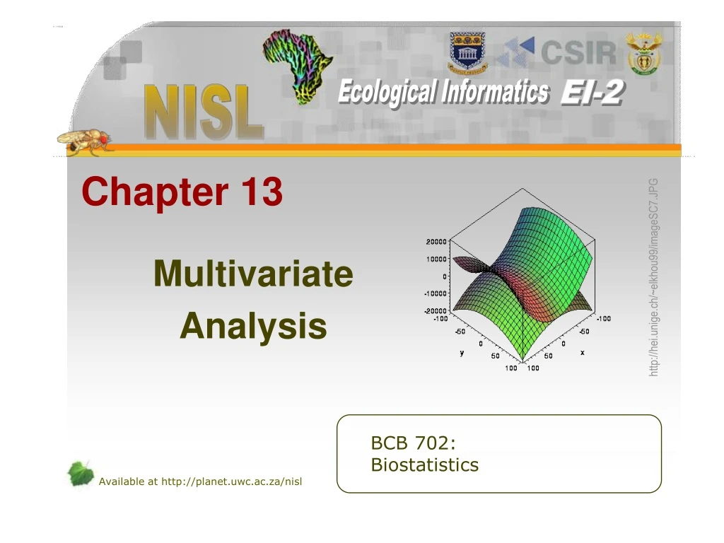
Chapter 13 Multivariate Analysis BCB 702: Biostatistics http://hei.unige.ch/~elkhou99/imageSC7.JPG
What is Multivariate Analysis? • Usually involves situations where there are two or more dependent (response) variables • Examines the relationships or interactions of these variables • Takes into account the fact that: • Variables may not be independent of each other • Performing multiple comparisons increases the risk of making a Type I error • Simply performing a series of multiple univariate tests would not be appropriate and would give false results
Types of Multivariate Tests Include: • Multivariate Analysis of Variance (MANOVA) • Discriminant Function Analysis (DFA) • Principal Components Analysis (PCA) • Factor Analysis • Cluster Analysis • Canonical Correlation Analysis • Multidimensional Scaling
MANOVA • Extension of the ANOVA • Examines two or more response variables • Combines multiple response variables into a single new variable to maximise the differences between the treatment group means • Obtain a multivariate F value – Wilks’ lambda (value between 0 and 1) is most commonly used • If the overall test is significant, we can then go on to examine which of the individual variables contributed to the significant effect
MANOVA: Example • A researcher has collected a certain species of lizard from three different island populations. Each island represents a different eco-zone. He wishes to test whether lizards from different islands differ in their morphology and abilities, so he collects 10 lizards from each island and measures their body length, limb length and running speed. • Independent variable: • Island of origin • Dependent variables: • Body length • Limb length • Running speed http://www.flickr.com/photos/wyscan/14739853/
MANOVA: Example • From the analysis, we get: • The model shows a significant difference in lizards from the three islands (p <0.001)
MANOVA: Example • Limb length and running speed differ significantly between lizards from different islands. There is no difference in body length
Discriminant Function Analysis • Discriminant Function Analysis (DFA) is used to determine which variables predict naturally occurring groups in data • Several independent variables and one non-metric (grouping) dependent variable • MANOVA in reverse • DFA organises the original independent variables into a set of canonical correlations, which are linear combinations of the original variables
Discriminant Function Analysis • The first canonical correlation explains the most variation in the data set, the second canonical correlation explains the most variation that is left over, and so on • Three steps: • Look for an overall significant effect using a multivariate F test (Wilks’ lambda) • Examine the independent variables individually for differences in mean by group • Classification
DFA: Example • Populations of a sunflower species grow at four sites (two in riparian habitat and two in serpentine habitat) that differ in soil chemistry and water availability. Various measures of soil chemistry were taken in order to determine which of these variables can be used to distinguish among sites. (Sambatti & Rice, 2006) • Independent variables: • Ca • Mg • P • Organic matter (OM) • pH • Dependent variable: • Site http://en.wikipedia.org/wiki/Image:Sunflowers.jpg
Canonical Centroid plot DFA: Example • The overall model was significant (p <0.001), meaning that sites differ in soil nutrients • First canonical axis: The riparian habitats (particularly R1) have more OM and a lower pH • Second canonical axis: The two serpentine habitats (S1 and S2) have lower levels of Ca and P and slightly higher levels of Mg than riparian sites
Principal Components Analysis • The goal of PCA is to reduce complex data sets containing a large number of variables to a lower dimension in order to see the relationships of variables more clearly • It computes a new set of composite variables called principal components (PCs) • Each PC explains a certain proportion of the variation in the data set, with PC1 explaining the most amount of variation, PC2 the next most amount of variation, and so on
Factor Analysis • Similar to Principal Components Analysis • Used to uncover underlying trends and relationships in large and complex data sets • Works on a correlation matrix of variables • Combines original variables into a smaller set of factors • Variables are correlated with each other due to their correlation with a common factor
A B C D E Cluster Analysis • Cluster analysis encompasses a number of different methods • Used to organize or group data according to similarities • There is no real dependent variable – cluster analysis does not attempt to explain why groups (clusters) exist • Often used in species taxonomy
Canonical Correlation Analysis • Used when variables fall naturally into two groups (a group of dependent variables and a group of independent variables) • Tries to determine if there are linear relationships between the two sets of variables • It creates functions for each group, such that the correlation between the functions of each group is maximised • In this way, a combination of variables from the first group predicts a combination of variables from the second group
Multidimensional Scaling • Analyses pairwise similarities between variables • Only applicable to continuous data • Plots variables graphically to provide a visual representation of the pattern of proximity of a set of variables (objects) • Objects plotted close together are relatively similar to each other, while objects plotted far apart are relatively dissimilar
