Vector Visualization

1. VectorVisualization Mengxia Zhu

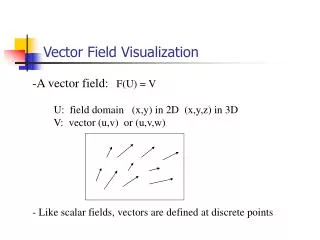
2. Vector Data • A vector is an object with direction and length v = (vx,vy,vz) • A vector field is a field which associates a vector with each point in space • The vector data is 3D representation of direction and magnitude • Examples include Fluid flow, velocity v Electromagnetic field, E, B Gradient of any scalar field A = T

3. Vector Field Visualization Techniques Local technique:Advection based methods - Display the trajectory starting from a particular location Global technique: Hedgehogs, Line Integral Convolution, Texture Splats etc. Display the flow direction everywhere in the field

4. Vector Field Viz Applications Computational Fluid Dynamics Weather modeling

5. Vector Field Visualization Challenges General Goal: Display the field’s directional information Domain Specific: Detect certain features Vortex cores, Swirl

6. Point Icons • • • • Draw point icons at selected points of the vector field • A natural approach is to draw an oriented, scaled line for each vector v = (vx,vy,vz) • The line begins at the point with which the vector is associated and is oriented in the direction of the vector components Arrows are added to indicate the direction of the line Lines may be colored according to the vector magnitude or type of the quantity (e.g. temperature) • Oriented glyphs (such as triangle or cone) can be used • To avoid visual clutter, the density of displayed icons must be kept very low • Point icons are useful in visualizing 2D slices of 3D vector fields •

7. Line Icons • Line icons provide a continuous representation of the vector field, thus avoiding interpolation of point icons • Line icons are particles traces, streaklines, and streamlines • In general, these three families of trajectories are distinct from each other • turbulent flows where flow pattern is time dependent • But they are equivalent to each other in steady flows

8. Air Flow over Windshield Air flow coming from a dashboard vent and striking the windshield of an automobile http://www-fp.mcs.anl.gov/fl

9. Particle Traces or Pathlines Final position • • • are trajectories traversed by fluid particles over time • An animation over time can give an illusion of motion • are computed by integrating • with initial condition x(0) = x0 • v(x,t) is a vector field wherexis the position • in space and t is time • Accuracy of numerical integration is crucial • give a sense of complete time evolution of the flow • are experimentally visualized by injecting instantaneously a dye or smoke in the flow and taking a long exposure photograph • • • • • • Initial position • simplest form Runge-Kutta of higher order can be used

10. Streaklines ti= t0 • • A streakline is the locus at time t0 of all the fluid particles that have previously passed through a specified point x0 • Line connecting particles released from the same location • is computed by linking the endpoints of all trajectories between times ti and t0 for every ti such that 0 ≤ ti ≤ t0 • gives information on the past history of the flow • is experimentally observed by injecting continuously at the point x0 a tracer such as hydrogen bubbles and by taking a short exposure photograph at time t0 • • • • • x0 • 0 ≤ ti ≤ t0 ti= 0 All particles passed through point x0 in the field

11. Streamlines or Fieldlines • are integral curves satisfying • where s is a parameter measuring the distance along the path • are everywhere tangent to the steady flow • provide an instantaneous picture of the flow at time t0 • are experimentally visualized by injecting a large number of tracer particles in the flow and taking a short-time exposure photograph at t0 curve s(x,t)

12. Streamlines through a Room Streamlines are color coded to display pressure variation

13. Streamlines (cont’d) - Displaying streamlines is a local technique because you can only visualize the flow directions initiated from one or a few particles - When the number of streamlines is increased, the scene becomes cluttered - You need to know where to drop the particle seeds - Streamline computation is expensive

14. Streamribbons • Are narrow surfaces defined by two adjacent streamlines and then bridging the lines with a polygonal mesh • Provide information about two flow parameters Vorticity (w)- a measure of rotation of the vector field • streamwise vorticity (Ω) is rotation of the vector field around the streamline and is depicted by the twist of the ribbon. Divergence - a measure of the spread of the flow • Changing width is proportional to the cross-flow divergence • Adjacent streamlines in divergent flows tend to spread. If too wide and must be discarded because the twist rate in the widely separated streamlines no longer reflect the vorticity along the trajectory

15. Streamtube • The combined effects of divergence and vorticity can be visualized in streamtubes which are effectively formed by linking a number (N) of streamribbons. Another way of generating the tube is to sweep an N-sided polygon along the streamline. • The rotation of the edges found in the tube represents streamwise vorticity, and the cross-section encodes cross flow divergence.

16. Streamtube Through a Room A single streamtube with diameter of the tube indicating flow-velocity, and color representing pressure variation. A thinner tube indicates faster flow.

17. Streampolygons • streampolygon is a regular polygon with n sides and radius r. • The goal of the streampolygon technique is to represent information about local strain (shear and convergence or divergence) and rotation in addition to the usual flow direction and velocity. • A polygon is placed into a vector field at a specified point and then deformed according to local strain • Align the polygon normal with the local vector • Rigid body rotation about the local vector is thus the streamwise vorticity • The radius of the polygon provides an additional degree of freedom and can be associated with some scalar value, Normal strain Shear strain Rotation Total deformation

18. Line Integral Convolution (LIC) LIC represents a new and general method for imaging two and three dimensional vector fields. The LIC Algorithm takes as : • Input: • An input texture image • A vector field • Output: generates an output image by filtering the input image along local stream lines defined by the vector field . • LIC emulates the effect of a strong wind blow across a fine sand.

19. DDA Convolution • This approach is a generalization of traditional line drawing techniques and the spatial convolution algorithms given by Van Wijk and Perlin.

20. DDA Convolution algorithm • Each vector in the field is used to define a long, narrow, DDA generated filter kernel that is tangential to the vector and going in the positive and negative vector direction some fixed distance, L. • A texture is then mapped one-to-one onto the vector field. • The input texture pixels under the filter kernel are summed, normalized by the length of the filter kernel, 2L, and placed in an output pixel image for the vector position.

21. DDA convolution example • l

22. Images generated by DDA . Simple circular vector field Computational fluid dynamics Input texture: white noise

23. DDA Drawback • Symmetry • This algorithm is very sensitive to symmetry of the DDA algorithm and filter. • If the algorithm weights the forward direction more than the backward direction, the circular field appear to spiral inward implying a vortical behavior that is not present in the field. • Accuracy • This algorithm assumes that the local vector field can be approximated by a straight line. • For complex structures smaller than the length of the DDA line, the local radius of curvature is small and is not well approximated by a straight line. • In a sense, DDA convolution renders the vector field unevenly, treating linear portions of the vector field more accurately than small scale vortices.

24. LIC • The LIC algorithm is a derivative of the DDA technique that, instead of using a vector, uses a local streamline to generate the filter. • The local behavior of the vector field can be approximated by computing a local stream line that starts at the center of pixel (x, y) and moves out in the positive and negative directions.  

25. As with the DDA algorithm, it is important to maintain symmetry about a cell. Hence, the local stream line is also advected backwards by the negative of the vector field as shown in equation (3). Negative Direction Primed variables represent the negative direction counterparts to the positive direction variables and are not repeated in subsequent definitions. As above Dsi, is always positive.

26. Illustration of local stream line calculation • Continuous sections of the local stream line — i.e. the straight line segments can be thought of as parameterized space curves. • The input texture pixel mapped to a cell can be treated as a continuous scalar function of x and y. • It is then possible to integrate over this scalar field along each parameterized space curve.

27. The entire LIC for output pixel F’(x, y) .

28. : Local Stream line L • The length of the local stream line, 2L, is • given in unit pixels. Depending on the input pixel field, F, if L is too large, all the resulting LICs will return values very close together for all coordinates (x, y). • On the other hand, if L is too small then an insufficient amount of filtering occurs. Since the value of L dramatically affects the performance of the algorithm, the smallest effective value is desired.

29. The effect of varying L

30. Application : • The LIC implementation is a module in a data flow system like that found in a number of public domain and commercial products. • This implementation allows for rapid exploration of various combinations of operators. The algorithm can be used as a data operator in conjunction with other operators. • Specifically, both the texture and the vector field can be preprocessed and combined with post processing on the output image.

31. Post processing: • The output of the LIC algorithm can be operated on in a variety of ways. In this section several standard techniques are used in combination with LIC to produce novel results.

32. . The fixed normalization fluid dynamics field is multiplied by a color image of the magnitude of the vector field.

33. A wind velocity visualization is created by compositing an image of North America under an image of the velocity field rendered using variable length LIC over 1/f noise.

34. Reference • This set of slides are developed from the lecture slides used by Prof. Karki at Louisiana State University. • Also from Prof. Jian Huang at University of Tennessee at Knoxville.