Download
1 / 46
540 likes | 924 Views
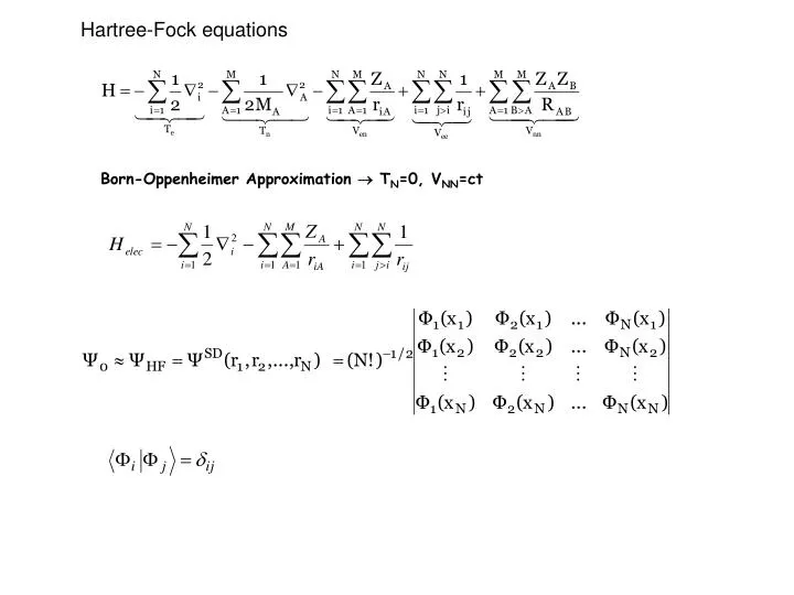
Hartree-Fock equations. Born-Oppenheimer Approximation T N =0, V NN =ct. - Core integral (one-electron integral. - Coulombian integral (two-electron integral). - Exchange integral (two-electron integral).

E N D
Hartree-Fock equations Born-Oppenheimer Approximation TN=0, VNN=ct
- Core integral (one-electron integral - Coulombian integral (two-electron integral) - Exchange integral (two-electron integral) Looking for the spin-orbitals which give the best EHF under the orthonormalization conditions and using the method of the Lagrange multipliers one obtains (see Jensen pg.62-63)
Hartree-Fock equations Lagrangean multipliers are eigenvalues of the Fock operator: - one-electron operator • Hartree-Fock potential • The average repulsive potential experienced by the i-th electron due to the remaining N-1 electrons • Replaces the complicated 1/r12 two-electron operator (electron-electron repulsion is taken into account only in an average way)
With: - represents the average local potential at position x1 arising from an electron located in j Operating with Jj(x1) we obtain: depends only on the value of i(x1) Jj is a local operator The second term of vHF(x1) is the exchange contribution to the Hartree-Fock potential: Kj(x1) exchanges the variables of the two spin-orbitals depends on the value of i on all points in space because it depends on the integrating variable Kj(x1) is a non-local operator JijKij0 Jii=Kii no self interaction in Hartree-Fock approximation
Conv.? Since fi depends on i HF equations must be solved iteratively (SCF procedure) No Initial guess vHF, f {i} Yes SD, EHF Molecular orbital energies: Total energy:
For a closed-shell system in RHF formalism, the total energy and molecular orbital energies are given by (see Szabo and Ostlund, pag.83): • Each occupied spin-orbital i contributes a term Hi to the energy • Each unique pair of electrons (irrespective of their spins) in spatial orbitals i and j contributes the term Jij to the energy • Each unique pair of electrons with parallel spins in spatial orbitals ψi and ψj contributes the term –Kij to the energy Examples: 3 2 1 a) b) c) d) a) E=2H1+J12 b) E=H1+H2+J12-K12 c) E=H1+H2+J12 d) E=H1+2H2+H3+2J12+J22+J13+2J23-K12-K13-K23
Koopmans’ Theorem What is the physical meaning of orbital energies? Total electronic energy: Summing all εi: why? because εi includes the Coulombian and exchange interactions with all the other electrons (also with εj). Similarly, εj will include also the interactions with εi, so that the interaction between the i-th and j-th electrons will be counted twice in the sum over orbital energies So, what εi is? Consider the ionization of the molecule (one electron removed from orbital number k) and suppose that no change of MO’s occurs during the ionization process
Koopmans’ theorem vertical ionization potential (IP) photoelectron spectroscopy (obtained without optimizing the cation geometry) adiabatic ionization potential is obtained when the geometry of the cation is optimized physical meaning of εi: the i-th orbital ionization energy!
Hartree-Fock-Roothaan Equations LCAO-MO i=1,2,...,K {μ} – a set of known functions The more complete set {μ}, the more accurate representation of the exact MO, the more exact the eigenfunctions of the Fock operator The problem of calculating HF MO the problem of calculating the set cμi LCAO coefficients matrix equation for the cμi coefficients Multiplying by μ*(r1) on the left and integrating we get: - Fock matrix (KxK Hermitian matrix) - overlap matrix (KxK Hermitian matrix) - Roothaan equations
More compactly: FC=SC where • the matrix of the expansion coefficients • (its columns describes the molecular orbitals) The requirement that the molecular orbitals be orthonormal in the LCAO approximation demands that: The problem of finding the molecular orbitals {i} and orbital energies i involves solving the matrix equation FC=SC. For this, we need an explicit expression for the Fock matrix
Charge density For a closed shell molecule, described by a single determinant wave-function The integral of this charge density is just the total number of electrons: Inserting the molecular orbital expansion into the expression for the charge density we get:
- elements of the density matrix • the electronic population of the atomic overlap distribution • give an indication of contributions to chemical binding when and • centered on different atoms - the net electronic charges residing in orbital Where: The integral of (r) is By means of the last equation, the electronic charge distribution may be decomposed into contributions associated with the various basis functions of the LCAO expansion. Off-diagonal elements Diagonal elements
Population analysis ≡ allocate the electrons in the molecule in a fractional manner, among the various parts of the molecule (atoms, bonds, basis functions) - Mulliken population analysis Substituting the basis set expansion we get: Basis set functions are normalized Sμμ=1 Pμμ - number of electrons associated with a particular BF - net population of φμ Qμ = 2PμSμ (μ≠)overlap population associated with two basis functions which may be on the same atom or on two different atoms Total electronic charge in a molecule consists of two parts: first term is associated with individual BF second term is associated with pairs of BF
- gross population for φμ the net charge associated with the atom A total overlap population between atoms A and B
Formaldehyde Mulliken population analysis #P RHF/STO-3G scf(conventional) Iop(3/33=6) Extralinks=L316 Noraff Symm=Noint Iop(3/33=1) pop(full) Basis functions:
= sum over the line (or column) corresponding to the C(1s) basis function = sum over the line (or column) corresponding to the O(2px) basis function
Atomic populations (AP) 1 O 8.186789 2 C 5.926642 3 H 0.943285 4 H 0.943285 Total atomic charges (Q=Z-AP) 1 O -0.186789 2 C 0.073358 3 H 0.056715 4 H 0.056715
Basis Sets with: {μ} – a set of known functions for UHF wave-functions two sets of coefficients are needed: if μ AO LCAO-MO if μ AO LCBF-MO
Basis functions • mathematical functions designed to give the maximum flexibility to the molecular orbitals • must have physical significance • their coefficients are obtained variationally
Slater Type Orbitals (STO) - similar to atomic orbitals of the hydrogen atom - more convenient (from the numerical calculation point of view) than AO, especially when n-l≥2 (radial part is simply r2, r3, ... and not a polinom) STO – are labeled like hydrogen atomic orbitals and their normalized form is: • STO • provide reasonable representations of atomic orbitals • however they are not well suited to numerical (fast) calculations of especially two-electron integrals • their use in practical molecular orbital calculations has been limited
STO • Advantages: • Physically, the exponential dependence on distance from the nucleus is very close to the exact hydrogenic orbitals. • Ensures fairly rapid convergence with increasing number of functions. • Disadvantages: • Three and four center integrals cannot be performed analytically. • No radial nodes. These can be introduced by making linear combinations of STOs. • Practical Use: • Calculations of very high accuracy, atomic and diatomic systems. • Semi-empirical methods where 3- and 4-center integrals are neglected.
Gaussian Type Orbitals (GTO) • introduced by Boys (1950) • powers of x, y, z multiplied by • α is a constant (called exponent) that determines the size (radial extent) of the function or: • N - normalization constant • f - scaling factor • scale all exponents in the related gaussians in molecular calculations l, m, n are not quantum numbers L=l+m+n - used analogously to the angular momentum quantum number for atoms to mark functions as s-type (L=0), p-type (L=1), d-type (L=2), etc (shells)
The absence of rn-1 pre-exponential factor restricts single gaussian primitives to approximate only 1s, 2p, 3d, 4f, ... orbitals. However, combinations of gaussians are able to approximate correct nodal properties of atomic orbitals GTO – uncontracted gaussian function (gaussian primitive) - contracted gaussian function (gaussian contraction) STO= GTOs are inferior to STOs in three ways: GTO’s behavior near the nucleus is poorly represented. At the nucleus, the GTO has zero slope; the STO has a cusp. GTOs diminish too rapidly with distance. The ‘tail’ behavior is poorly represented. Extra d-, f-, g-, etc. functions (from Cart. rep.)may lead to linear dependence of the basis set. They are usually dropped when large basis sets are used. Advantage: GTOs have analytical solutions. Use a linear combination of GTOs to overcome these deficiencies.
There are 6 possible d-type cartesian gaussians while there are only 5 linearly independent and orthogonal d orbitals The gs, gx, gy and gz primitives have the angular symmetries of the four corresponding AO. The 6 d-type gaussian primitives may be combined to obtain a set of 5 d-type functions: gxy dxy gxz dxz gyz dyz The 6-th linear combination gives an s-type function: In a similar manner, the 10 f-type gaussian primitives may be combined to obtain a set of 7 f-type functions
GTOs are less satisfactory than STOs in describing the AOs close to the nucleus. The two type functions substantially differ for r=0 and also, for very large values of r. cusp condition: for STO: [d/dr e-ξr]r ≠ 0 for GTO: With GTO the two-electron integrals are more easily evaluated. The reason is that the product of two gaussians, each on different centers, is another gaussian centered between the two centers: where: KAB=(2αβ/[(α+β)π])3/4exp(-αβ/(α+β)|RA-RB|2] The exponent of the new gaussian centered at Rp is: p=α+β and the third center P is on line joining the centers A and B (see the Figure below) RP=(αRA+βRB)/(α+β)
The product of two 1s gaussian is a third 1s gaussian allow a more rapidly and efficiently calculation of the two-electron integrals GTO have different functional behavior with respect to known functional behavior of AOs. contractions (CGF or CGTO) L – the length of the contraction dpμ – contraction coefficients
How the gaussian primitives are derived? • by fitting the CGF to an STO using a least square method • varying the exponents in quantum calculations on atoms in order to minimize the energy Example STO-3G basis set for H2 molecule Each BF is approximated by a STO, which in turn, is fitted to a CGF of 3 primitives hydrogen 1s orbital in STO-3G basis set For molecular calculations, first we need a BF to describe the H 1s atomic orbital then: MO(H2) = LCBF 3 gaussian primitives: exponent coefficient 0.222766 0.154329 0.405771 0.535328 0.109818 0.444636 If we use a scaling factor:
βi=αif2 ! Using normalized primitives we do not need a normalization factor for the whole contraction If the primitives are not normalized, we have to obtain a normalization factor. For this we use the condition: S=F2[I1+I2+I3+2I4+2I5+2I6]
But: so that: Analogously: and thus:
Now, Imposing that S=1 we obtain: In the general case of a contraction of dimension n, the above expression become:
Summary The 1s hydrogen orbital in STO-3G basis set will be: with: - normalization factors for primitives - normalization factor for the whole contraction (when un-normalized primitives or segmented contractions are used) N=1.0000002
Explicitly: If the exponents are not scaled:
STO-3G basis set example http://www.chem.utas.edu.au/staff/yatesb/honours/modules/mod5/c_sto3g.html This is an example of the STO-3G basis set for methane in the format produced by the "gfinput" command in the Gaussian computer program. The first atom is carbon. The other four are hydrogens. Standard basis: STO-3G (5D, 7F) Basis set in the form of general basis input: 1 0 S 3 1.00 .7161683735D+02 .1543289673D+00 .1304509632D+02 .5353281423D+00 .3530512160D+01 .4446345422D+00 SP 3 1.00 .2941249355D+01 -.9996722919D-01 .1559162750D+00 .6834830964D+00 .3995128261D+00 .6076837186D+00 .2222899159D+00 .7001154689D+00 .3919573931D+00 **** 2 0 S 3 1.00 .3425250914D+01 .1543289673D+00 .6239137298D+00 .5353281423D+00 .1688554040D+00 .4446345422D+00 **** 3 0 S 3 1.00 .3425250914D+01 .1543289673D+00 .6239137298D+00 .5353281423D+00 .1688554040D+00 .4446345422D+00 **** 4 0 S 3 1.00 .3425250914D+01 .1543289673D+00 .6239137298D+00 .5353281423D+00 .1688554040D+00 .4446345422D+00 **** 5 0 S 3 1.00 .3425250914D+01 .1543289673D+00 .6239137298D+00 .5353281423D+00 .1688554040D+00 .4446345422D+00 ****
Split valence basis sets http://www.chem.utas.edu.au/staff/yatesb/honours/modules/mod5/split_bas.html Valence orbitals are represented by more than one basis function, (each of which can in turn be composed of a fixed linear combination of primitive Gaussian functions). Depending on the number of basis functions used for the reprezentation of valence orbitals, the basis sets are called valence double, triple, or quadruple-zeta basis sets. Since the different orbitals of the split have different spatial extents, the combination allows the electron density to adjust its spatial extent appropriate to the particular molecular environment. Split is often made for valence orbitals only, which are chemically important. 3-21G basis set The valence functions are split into one basis function with two GTOs, and one with only one GTO. (This is the "two one" part of the nomenclature.) The core consists of three primitive GTOs contracted into one basis function, as in the STO-3G basis set. 1 0 //C atom S 3 1.00 .1722560000D+03 .6176690000D-01 .2591090000D+02 .3587940000D+00 .5533350000D+01 .7007130000D+00 SP 2 1.00 .3664980000D+01 -.3958970000D+00 .2364600000D+00 .7705450000D+00 .1215840000D+01 .8606190000D+00 SP 1 1.00 .1958570000D+00 .1000000000D+01 .1000000000D+01 **** 2 0 //H atom S 2 1.00 .5447178000D+01 .1562850000D+00 .8245472400D+00 .9046910000D+00 S 1 1.00 .1831915800D+00 .1000000000D+01 **** 6-311G basis set
Extended basis sets The most important additions to basis sets are polarization functions and diffuse basis functions. Polarization basis functions The influence of the neighboring nuclei will distort or polarize the electron density near a given nucleus. In order to take this effect into account, orbitals that have more flexible shapes in a molecule than the s, p, d, etc shapes in the free atoms are used. An s orbital is polarized by using a p-type orbital A p orbital is polarized by mixing in a d-type orbital 6-31G(d) a set of d orbitals is used as polarization functions on heavy atoms 6-31G(d,p) a set of d orbitals are used as polarization functions on heavy atoms and a set of porbitals are used as polarization functions on hydrogen atoms
Diffuse basis functions For excited states and anions where the electronic density is more spread out over the molecule, some basis functions which themselves are more spread out are needed (i.e. GTOs with small exponents). These additional basis functions are called diffuse functions. They are normally added as single GTOs. 6-31+G - adds a set of diffuse sp orbitals to the atoms in the first and second rows (Li - Cl). 6-31++G - adds a set of diffuse sp orbitals to the atoms in the first and second rows (Li- Cl) and a set of diffuse s functions to hydrogen. Diffuse functions can also be added along with polarization functions. This leads, for example, to the 6-31+G(d), 6-31++G(d), 6-31+G(d,p) and 6-31++G(d,p) basis sets. Standard basis: 6-31+G (6D, 7F) Basis set in the form of general basis input: 1 0 S 6 1.00 .3047524880D+04 .1834737130D-02 .4573695180D+03 .1403732280D-01 .1039486850D+03 .6884262220D-01 .2921015530D+02 .2321844430D+00 .9286662960D+01 .4679413480D+00 .3163926960D+01 .3623119850D+00 SP 3 1.00 .7868272350D+01 -.1193324200D+00 .6899906660D-01 .1881288540D+01 -.1608541520D+00 .3164239610D+00 .5442492580D+00 .1143456440D+01 .7443082910D+00 SP 1 1.00 .1687144782D+00 .1000000000D+01 .1000000000D+01 SP 1 1.00 .4380000000D-01 .1000000000D+01 .1000000000D+01 **** 2 0 S 3 1.00 .1873113696D+02 .3349460434D-01 .2825394365D+01 .2347269535D+00 .6401216923D+00 .8137573262D+00 S 1 1.00 .1612777588D+00 .1000000000D+01 ****
Number of primitives and basis functions for 1,2-Benzosemiquinone free radical with the STO-3G basis set Primitives: atom C: nr.primitives = 15 x nr. atoms = 6 → 90 atom H: nr.primitives = 3 x nr. atoms = 4 → 12 atom O: nr.primitives = 15 x nr. atoms = 2 → 30 TOTAL: 132 GTO primitives Basis functions: atom C: nr. BF = 5 x nr.atoms = 6 → 30 atom H: nr. BF = 1 x nr.atoms = 4 → 4 atom O: nr. BF = 5 x nr.atoms = 2 → 10 TOTAL: 44BF
Number of primitives and basis functions for 1,2-Benzosemiquinone free radical with the 6-31+G* (6-31+G(d)) basis set Primitives: atom C: nr.primitives = 32 x nr. atoms = 6 → 192 atom H: nr.primitives = 4 x nr. atoms = 4 → 16 atom O: nr.primitives = 32 x nr. atoms = 2 → 64 TOTAL: 272 GTO primitives Basis functions: atom C: nr. BF = 19 x nr.atoms = 6 → 114 atom H: nr. BF = 2 x nr.atoms = 4 → 8 atom O: nr. BF = 19 x nr.atoms = 2 → 38 TOTAL: 160BF
Effective core potentials (ECPs) • Core electrons, which are not chemically very important, require a large number of basis functions for an accurate description of their orbitals. • An effective core potential is a linear combination of specially designed Gaussian functions that model the core electrons, i.e., the core electrons are represented by a effective potential and one treats only the valence electrons explicitly. • ECP reduces the size of the basis set needed to represent the atom (but introduces additional approximations) • for heavy elements, pseudopotentials can also include of relativistic effects that otherwise would be costly to treat ECP potentials are specified as parameters of the following equation: where p is the dimension of the expansion di are the coefficients for the expansion terms, r0 is the distance from nucleus and ξi represents the exponents for each term. • Saving computational effort • Taking care of relativistic effects partly • Important for heavy atoms, e.g., transition metal atoms
ECP example complexPd1.chk #P Opt B3LYP/gen pseudo=read complex Pd v1 0 2 C 8.89318310 9.90388210 6.72569337 C 9.52931379 8.77525770 6.27102032 H 9.29586123 7.93893890 6.60431879 C 10.52592748 8.89096200 5.30965653 H 10.95942133 8.13380930 4.98695425 C 10.85850598 10.13123090 4.84438728 H 11.51852449 10.22866610 4.19609286 C 10.20972534 11.23549650 5.34144511 etc. etc. H 4.15752044 17.83312399 10.48668123 H 5.63848578 17.14049639 11.10318367 N C O H 0 6-31G(d) **** Pd 0 CEP-121G **** Pd 0 CEP-121G • Recomendations for basis set selection • Always a compromise between accuracy and computational cost! • With the increase of basis set size, calculated energy will converge (complete basis set (CBS) limit). • Special cases (anion, transition metal, transtion state) • Use smaller basis sets for preliminary calculations and for heavy duties (e.g., geometry optimizations), and use larger basis sets to refine calculations. • Use larger basis sets for critical atoms (e.g., atoms directly involved in bond-breaking/forming), and use smaller basis sets for unimportant atoms (e.g., atoms distant away from active site). • Use popular and recommended basis sets. They have been tested a lot and shown to be good for certain types of calculations.