Feedback 101
Feedback 101. Stuart Henderson. March 15-18, 2004. Outline. Introduction to Feedback Block diagram Uses of feedback systems (dampers, instabilities, longitudinal, transverse System requirements Resources (paper) Simplest feedback system scheme Ideal conditions

Feedback 101
E N D
Presentation Transcript
Feedback 101 Stuart Henderson March 15-18, 2004
Outline Introduction to Feedback Block diagram Uses of feedback systems (dampers, instabilities, longitudinal, transverse System requirements Resources (paper) Simplest feedback system scheme Ideal conditions Eigenvalue problem and solution Loop delay, delayed kick Closed-orbit problem Filtering schemes (analog/digital) Two turn filtering scheme Type of digital filters (FIR, IIR) Kickers Concepts Dp and dtheta calculation Figures of merit Plots of freq response, etc. Complete System Response Estimates for damping e-p RF amplifiers Parameters, cost, etc. Feedback in the ORBIT code
Resources • Several good overviews and papers on feedback systems and kickers: • Pickups and Kickers: • Goldberg and Lambertson, AIP Conf. Proc. 249, (1992) p.537 • Feedback Systems: • F. Pedersen, AIP Conf. Proc. 214 (1990) 246, or CERN PS/90-49 (AR) • D. Boussard, Proc. 5th Adv. Acc. Phys. Course, CERN 95-06, vol. 1 (1995) p.391 • J. Rogers, in Handbook of Accelerator Physics and Technology, eds. Chao and Tigner, p. 494.
Why Feedback Systems? • High intensity circular accelerators eventually encounter collective beam instabilities that limit their performance • Once natural damping mechanisms (radiation damping for e+e- machines, or Landau damping for hadron machines) are insufficient to maintain beam stability, the beam intensity can no longer be increased • There are two potential solutions: • Reduce the offending impedance in the ring • Provide active damping with a Feedback System • A Feedback System uses a beam position monitor to generate an error signal that drives a kicker to minimize the error signal • If the damping rate provided by the feedback system is larger than the growth rate of the instability, then the beam is stable. • The beam intensity can be increased until the growth rate reaches the feedback damping rate
Types of Feedback Systems • Feedback systems are used to damp instabilities • Typical applications are bunch-by-bunch feedback in e+e- colliders, hadron colliders to damp multi-bunch instabilities • Dampers are used to damp injection transients, and are functionally identical to feedback systems • These are common in circular hadron machines (Tevatron, Main Injector, RHIC, AGS, …) • Feedback systems and Dampers are used in all three planes: • Transverse feedback systems use BPMs and transverse deflectors… • Longitudinal feedback systems use summed BPM signals to detect beam phase, and correct with RF cavities, symmetrically powered striplines,…
Elements of a Feedback System • Basic elements: • Pickup • Signal Processing • RF Power Amplifier • Kicker • Pickup is BPM for transverse, phase detector for longitudinal • Processing scheme can be analog or digital, depending on needs • Transverse Kicker: • Low-frequency: ferrite-yoke magnet • High-frequency: stripline kicker • Longitudinal Kicker can be RF cavity or symmetrically powered striplines Signal Processing RF amp Kicker Pickup Beam
Specifying a Feedback System • Feedback systems are characterized by • Bandwidth (range of relevant mode frequencies) • Gain (factor relating a measured error signal to output corrective deflection) • Damping rate • In order to specify a feedback system for damping an instability, we must know • Which plane is unstable • Mode frequencies • Growth rates • RF power amplifier is chosen based on required bandwidth and damping rate. Typical systems use amplifiers with 10-100 MHz bandwidth, and 100-1000W output power.
Simple picture of feedback X • Take simple (but not very realistic) situation: • -functions at pickup and kicker are equal • 90 phase advance between kicker & pickup • Integer tune Position measurement (coordinates x, x’) X Kick (coordinates y, y’) • System produces a kick proportional to the measured displacement: • At the kicker: • At the BPM after 1 turn:
Simple picture of feedback, continued • So x-amplitude after 1 turn has been reduced by • Giving a rate of change in amplitude: • Giving a damping rate: • But, we don’t really operate with integer tune. Averaging over all arrival phases gives a factor of two reduction: • In real life, we may not be able to place the BPM and kicker 90 degrees apart in phase, and the locations will not have equal beta functions. We need a realistic calculation.
Realistic damping rate calculation for simple processing M2, 2 • Follow Koscielniak and Tran • Coordinates at pickup are (xn,xn) on turn n • Coordinates at kicker are (yn,yn) on turn n • Transport between pickup and kicker has 2x2 matrix M1 and phase 1 • Transport between kicker and pickup has 2x2 matrix M2 and phase 2 • Give a kick on turn n proportional to the position measured on the same turn: • Where G is the feedback gain Kicker (y,y) Pickup (x,x) M1, 1
Simple processing, cont’d • The coordinates one turn later are given by:
More realistic damping rate calculation, cont’d • After n turns the coordinates are • This is an eigenvalue problem with solution • The eigenvalues can be obtained from One-turn matrix
General solution for 2x2 real matrix • Since we have a 2x2 real matrix, we expect two eigenvalues which are complex conjugate pairs. Writing • Where we can identify as the damping rate (per turn), and as the tune, which in general will be modified by the feedback system • Solution: Giving,
Damping rate and tune shift for simple processing • We have • With p, p the twiss parameters at the pickup, k, k at the kicker, the tune, 1 the phase advance between pickup and kicker, 2 the phase advance from kicker around the ring to pickup: • Finally,
Damping rate and tuneshift for small damping • For weak damping, • And • Optimal damping rate results for 1=90 degrees turns-1 sec-1 radians
Finite Loop Delay • Up to this point we have ignored the fact that it takes time to “decide” on the kick strength in the processing electronics • It is not necessary to kick on the same turn • We can kick m turns later: • In this way we can “wait around” for the optimum turn to provide the optimum phase
Closed-Orbit Problem: the 2-turn filter • Our simplification ignores another problem: • A closed orbit error in the BPM will cause the feedback system to try to correct this closed orbit error, using up the dynamic range of the system • Solution: • Analog: a self-balanced front-end • Digital: Filter out the closed-orbit by using an error signal that is the difference between successive turns • 2-turn filter constructs an error signal:
2-turn filter, cont’d • With • The transfer function of the filter is: • This gives a “notch” filter at all the rotation harmonics, which are the harmonics that result from a closed orbit error
Kickers for Transverse Feedback Systems • For low frequencies (< 10 MHz), it is possible to use ferrite-yoke magnets, but the inductance limits their bandwidth • Broadband transverse kickers usually employ stripline electrodes • Stripline electrode and chamber wall form transmission line with characteristic impedance ZL
Stripline Kicker Layout +VL ZL ZL d Beam l ZL ZL -VL
Stripline Kicker Schematic Model Zc VK Beam Out Beam In p p+ p
Stripline Kicker Analysis +V • Deflection from parallel plates of length l, separated by distance d, at opposite DC voltages, +/- V is: • We need to account for the finite size of the plates (width w, separation d). A geometry factor g 1 is introduced: • Because we want to damp instabilities that have a range of frequencies, we will apply a time-varying potential to the plates V(). • We need to calculate the deflection as a function of frequency and beam velocity. -V
Deflection by Stripline Kicker • Stripline kicker terminated in a matched load produces plane wave propagating in +z direction between the plates. • For beam traveling in +z direction: • For beam traveling in –z direction: • For relativistic beams, we need the beam traveling opposite the wave propagation!
Deflection by Stripline Kicker • Where • This can be written in phase/amplitude form as:
Powering the Stripline Kicker • For transverse deflection, one could • Independently power each stripline with its own source • Power the pair of striplines from a single RF power source by splitting (e.g. with a 180 degree hybrid to drive electrodes differentially) • Using a matched splitting arrangement, the delivered power is: • Which equals the power dissipated on the two stripline terminations: • So that the input voltage is:
Figures of Merit for Stripline Kickers • One common figure of merit seen in the literature is the Kicker Sensitivity. • From which we get: • Which can be written in the form • Important points: • Deflection has a phase shift relative to the voltage pulse • sin/ shows the typical transit-time factor response
Transverse Shunt Impedance • In analogy with RF cavities, one can define an effective shunt impedance that relates the transverse “voltage” to the kicker power: • So after all this, what’s the kick?
Multiple Kickers • For N kickers, each driven with power P, • Where PT=NP is the total installed power • To achieve the same deflection (damping rate) with N kickers requires only • Example: One kicker with P1=1000W gives same kick as two kickers each driven at 250 W
Putting it all together • The RF power amplifier puts out full strength for a certain maximum error signal • The system produces the maximum deflection max for a maximum amplitude xmax • For optimal BPM/Kicker phase, the optimal damping rate is • For a Damper systems, xmax is large enough to accommodate the injection transient • For a Feedback system, xmax is many times the noise floor
Parameters for an e-p feedback system • Bandwidth: • Treat longitudinal slices of the beam as independent bunches • Ensure sufficient bandwidth to cover coherent spectrum • Choose 200 MHz • Damping time: • To completely damp instability, we need 200 turns • To influence instability, and realize some increase in threshold, perhaps 400 turns is sufficient • Input parameters: • y= 7 meters • Xmax = 2mm • Stripline length = 0.5 m, separation d = 0.10, w/d = 1.0