Computational Physics Numerical Differentiation
Computational Physics Numerical Differentiation. Dr. Guy Tel- Zur. Clouds. Picture by Peter Griffin, publicdomainpictures.net. MHJ Chapter 3: Numerical Differentiation. Should be f’c. “2” stands for two points. forward/backward 1 st derivative: ±h. N-points stencil. Example code.

Computational Physics Numerical Differentiation
E N D
Presentation Transcript
Computational PhysicsNumerical Differentiation Dr. Guy Tel-Zur Clouds. Picture by Peter Griffin, publicdomainpictures.net
MHJ Chapter 3: Numerical Differentiation Should be f’c “2” stands for two points
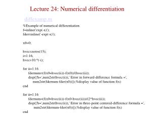
Example code • 2nd derivative of exp(x) • Code in C++, we will learn more of the language features: • Pointers • Call by Value/Reference • Dynamic memory allocation • Files (I/O)
Call by value vs. call by reference • printf(“speed= %d\n”, v); // this is a call by value as the value of v won’t be changed by the function (printf) – which is desired • scanf(“%d\n”,&v); // this is a call by reference, we want to supply the address of v in order to set it’s value(s)
ניתוח תכנית לדוגמה // // This program module // demonstrates memory allocation and data transfer in between functions in C++ #include<stdio.h> #include<stdlib.h> int main(intargc, char *argv[]) { inta; // line 1 int *b; // line 2 a = 10; // line 3 b = new int[10]; // line 4 for(i = 0; i < 10; i++) { b[i] = i; // line 5 } func( a,b); // line 6 return 0; } // End: function main() void func( int x, int *y) // line 7 { x += 7; // line 8 *y += 10; // line 9 y[6] += 10; // line 10 return; // line 11 } // End: function func()
// // This program module // demonstrates memory allocation and data transfer in between functions in C++ #include<stdio.h> #include<stdlib.h> void func( int x, int *y); int main(intargc, char *argv[]) { int a; // line 1 int *b; // line 2 a = 10; // line 3 b = new int[10]; // line 4 for(int i = 0; i < 10; i++) { b[i] = i; // line 5 } func( a,b); // line 6 printf("a=%d\n",a); printf("b[0]=%d\n",b[0]); printf("b[1]=%d\n",b[0]); printf("b[2]=%d\n",b[0]); printf("b[3]=%d\n",b[0]); printf("b[4]=%d\n",b[0]); printf("b[5]=%d\n",b[0]); printf("b[6]=%d\n",b[0]); printf("b[7]=%d\n",b[0]); printf("b[8]=%d\n",b[0]); printf("b[9]=%d\n",b[0]); return 0; } // End: function main() void func( int x, int *y) // line 7 { x += 7; // line 8 *y += 10; // line 9 y[6] += 10; // line 10 return; // line 11 } // End: function func() תכנית משופרת Check program: demo1.cpp Under /lectures/02/code
הנושאים שיידונו מכאן הלאה עד לסיום פרק 3 מתוך MHJ • תכנית מס' 1: חישוב הנגזרת השנייה של exp(x) בשפת C++ • תכנית מס' 2:תכנית דומה בשפת C בתוספת התיחסות לפתיחת קבצים לקריאה ולכתיבה • תכנית מס' 3: כמו תכנית מס' 2 אלא שהפעם בשפת C++ והדגשת השוני בינהן. • תכנית מס' 4: כנ"ל בשפת Fortran90 • דיון בהערכת השגיאה בחישוב • הצגה גראפית של השגיאה – תוכנת gnuplot
Self.Open( DevC++ for the demos!)תזכורת לעצמי • I slightly modified “program1.cpp” from MHJ section 3.2.1 (2009 Fall edition): http://www.fys.uio.no/compphys/cp/programs/FYS3150/chapter03/cpp/program1.cpp
Explain program1.cpp Working directory: C:\Users\telzur\Documents\BGU\Teaching\ComputationalPhysics\2011A\Lectures\02\code> Open DevC++ IDE for the demo Usage: > program1 <user input> 0.01 10 100 Examine the output: > type out.dat
program2.cpp • The book mentions program2.cpp which is in cpp and the URL is indeed a cpp code, but the listing below the URL is in C. • This demonstrates the I/O differences between C and C++
Working with files in C++ program2.cpp using namespace std; #include <iostream> int main(intargc, char *argv[]) { FILE *in_file, *out_file; if( argc < 3) { printf("The programs has the following structure :\n"); printf("write in the name of the input and output files \n"); exit(0); } in_file = fopen( argv[1], "r"); // returns pointer to the input file if( in_file == NULL ) { // NULL means that the file is missing printf("Can't find the input file %s\n", argv[1]); exit(0); } out_file = fopen( argv[2], "w"); // returns a pointer to the output file if( out_file == NULL ) { // can't find the file printf("Can't find the output file%s\n", argv[2]); exit(0); } fclose(in_file); fclose(out_file); return 0; }
program3.cpp • Usage: > program3 outfile_name • All the rest is like in program1.cpp
Now lets check the f90 version • Open in SciTEprogram1.f90 • In the image below: compilation and execution demo:
Content of exp(10)’’ computation • See MHJ section 3.2.2 and Fig. 3.2 (Fall 2009 Edition) • Text output with 4 columns: h, computed_derivative, log(h),ε >program1 Input: 0.1 10. 10 >more out.dat 1.00000E-001 2.72055E+000 -1.00000E+000 -3.07904E+000 5.00000E-002 2.71885E+000 -1.30103E+000 -3.68121E+000 2.50000E-002 2.71842E+000 -1.60206E+000 -4.28329E+000 1.25000E-002 2.71832E+000 -1.90309E+000 -4.88536E+000 6.25000E-003 2.71829E+000 -2.20412E+000 -5.48742E+000 3.12500E-003 2.71828E+000 -2.50515E+000 -6.08948E+000 1.56250E-003 2.71828E+000 -2.80618E+000 -6.69162E+000 7.81250E-004 2.71828E+000 -3.10721E+000 -7.29433E+000 3.90625E-004 2.71828E+000 -3.40824E+000 -7.89329E+000 1.95313E-004 2.71828E+000 -3.70927E+000 -8.44284E+000
Download and install Gnuplot http://www.gnuplot.info/
Visualization: Gnuplot • Reconstruct result from MHJ - Figure 3.2 using gnuplot • Gnuplot is included in Python(x,y) package! • Gnuplot tutorial: http://www.duke.edu/~hpgavin/gnuplot.html • Example: http://www.physics.ohio-state.edu/~ntg/780/handouts/gnuplot_quadeq_example.pdf • 3D Examples: http://www.physics.ohio-state.edu/~ntg/780/handouts/gnuplot_3d_example_v2.pdf
Can we explain this behavior? Computed for x=10
Error Analysis εro = Round-Off error The approximation error: Recall Eq. 3.4: The leading term in the error (j=1) is therefore:
The Round-Off Error (εro) • εrodepends on the precision level of the chosen variables (single or double precision) Single precision If the terms are very close the difference is at the level of the round off error Double precision
hmin = 10-4 is therefore the step size that gives the minimal error in our case. If h>hmin the round-off error term will dominate
Let’s upgrade our visualization skills! • Mayavi • Included in the Python(x,y) package • 2D/3D • User guide: http://code.enthought.com/projects/mayavi/docs/development/html/mayavi/index.html
A nice demo • Source: http://code.enthought.com/projects/mayavi/docs/development/html/mayavi/mlab.html#id5