Uncertainty in a GIS
320 likes | 788 Views
Uncertainty in a GIS. Brian Klinkenberg Geography 516. T o C. Spatial variability Data uncertainty I: measurement and sampling errors Representational uncertainty I: objects vs fields Representational uncertainty II: cartographic conventions Data uncertainty II: MAUP and S.A.

Uncertainty in a GIS
E N D
Presentation Transcript
Uncertainty in a GIS Brian Klinkenberg Geography 516
T o C • Spatial variability • Data uncertainty I: measurement and sampling errors • Representational uncertainty I: objects vs fields • Representational uncertainty II: cartographic conventions • Data uncertainty II: MAUP and S.A. • Rule uncertainty • Managing uncertainty: error propagation and MC simulation
Why an issue? • Basic search for the truth in science • Safeguard against litigation • Jurisdictional requirements for mandatory data quality reports • Protect individual and agency reputations • Touches everyone involved in GIS, from data producers to software and hardware vendors, to end users
Definition • Uncertainty: our imperfect and inexact knowledge of the world • Data: we are unsure of what exactly we observe or measure in society or nature • Rule: we are unsure of the conclusions we can draw from even perfect data (how we reason with the observations)
Spatial variability • Just about everything varies over space (spatial dependence). • Why? • Therefore, an estimation of uncertainty is important. The estimate can be: • Descriptive • Quantitative: • sensitivity analysis • Confidence limits (statistical or error propagation)
Spatial variability • The causes of natural phenomena vary in space (continental drift > mountains > rainy regions / rain shadows) • Therefore, so do the natural resources that depend on them; as do socio-economic processes. • E.g., Soil ≈ f(parent material, climate, organisms, topography, time, ….)
Spatial gradients • Four components: • Non-spatially structured environmental variation • Spatially-structured environmental variation • Spatial variation of the variable of interest that is not shared by the environmental variables • Unexplained, non-spatial variation
Data uncertainty IMeasurement and sampling errors • H0: The true value of a parameter is unknown. • Measurement errors: • Limited precision of our measuring devices • The typical concern of standard statistics • Errors are independent, normally distributed, exactly characterizable • Can characterize through repeated sampling and statistical characterization (I,ND)
Data uncertainty I • Mistakes • Systematic and random equipment problems • Data collection methods • Observer diligence and bias • Mismatch of data collected by different methods • In most GIS analyses those types of errors are usually insignificant relative to:
Data uncertainty I • Sampling uncertainty: • We almost always use a sample to collect data • To collect accurate samples requires extensive knowledge of the object (and its relations to other objects), knowledge we typically don’t have until after we sample • Sampling strategies: random, stratified, systematic (effects of spatial autocorrelation?) • Use GIS to predetermine sampling strategy (sampling framework) • Can quantify through repeated sampling, but $ and time often preclude such efforts
Data uncertainty I • In addition to the standard sampling issues, we should also consider: • Positional accuracy (x, y, z) • Semantic accuracy (does everyone agree what the term means) • If several variables are correlated (i.e., not independent), it is not sufficient to describe their univariate distribution. Instead, we must determine their multivariate distribution, which in general involves the computation of a variance-covariance matrix. This is much more difficult to establish than univariate distributions. • The covariance structure is important because if we compute a function of several variables, the uncertainty of the result depends not only on the individual variances of the variables, but also on their covariances.
Representation IObjects and Fields • Issue: GIS fosters the combination of disparate data sets, each of which may have a very different uncertainty structure associated with it. • How best to represent the data (uncertainty) so that the results best reflect the overall uncertainty?
Representation I • Points – not an issue, although scale can create problems • Areas: object or field representation? • Implies different sampling strategies and data conversion issues (raster <> vector) • Object: representing the map unit • a single representative value • Use mean / “expected value” • Loss of knowledge of variability within map unit, or of quality of estimate
Representation I • Using a range of values (classes; e.g., 0-3% slope) • Useful for sensitivity analyses • What is the expected value? • Using a statistical distribution • Should be able to completely describe the data values and their probability of being encountered • Problem: theoretical or observational justification • Using a non-parametric distribution • Based on repeated sampling of object • Makes no assumptions about distribution • Less statistical power
Representation I • Field: representing ‘continuous’ space • Requires sampling scheme • Compounded by rule uncertainty associated with spatially interpolating the points (lines & areas) into the ‘field’ (inverse-distance weighted, geostatistics, trend surface analysis, etc.) • Storage considerations (raster, TIN, ?)
Representation IICartographic presentation • Cartographic conventions / abstraction • Simplification, classification, induction, symbolization • Simplification: how to retain the character of the feature (fractals) • The effect of scale on the symbolization (most methods actually perform coordinate reduction, not entity simplification [coordinates are valued over topology]—e.g., Douglas and Poiker algorithm)
Representation II • As abstraction increases, rules change from quantitative (simple scale reduction by coordinate elimination) to qualitative (feature selection, exaggeration) • As the scale is reduced, features evolve from areal (wide rivers) to linear, from areal to point (cultural features), from being ‘to scale’ to gross exaggeration (roads)
Representation II • Typical problems: • Consider the Arctic, with its multitude of small lakes. An area may be 50% water, but as the scale is reduced the size of the individual lakes is such that they would not be represented on the map. That would lead to the impression that the area is devoid of water. What to do? • Consider the coast of BC, with its many fjords. As the map scale is reduced, most fjords have to be removed; otherwise no details would be visible. • Some cart notes on the subject.
Data uncertainty IIMAUP and S.A. • The modifiable areal unit problem and spatial autocorrelation create data uncertainty. • Gerrymandering example of MAUP:
Data uncertainty II • Spatial autocorrelation can create ‘false’ gradients in data: • In a ‘true’ gradient the value z observed at any location (i,j) can be expressed as a function of its geographic coordinates x & y plus an error term that is independent from location to location • Zij = b0 + b1xij + b2yij + εij
Data uncertainty II • In a true gradient, the error terms at neighbouring points are not correlated with one another. • A true gradient violates the stationarity assumption of most spatial-analysis methods because the expected value varies from place to place. It should be removed from the data before proceeding (e.g., trend surface analysis).
Data uncertainty II • In a “false” gradient, the observed trend is caused by spatial autocorrelation. • There is no change in the expected value throughout the area, although the observed value at each locality is partly determined by neighbouring values: • zij = b0 + ∑f(zij) + εij • where ∑f(zij) represents the sum of the effects of points located within some distance d from the value zij that we are trying to describe.
Data uncertainty II • If the gradient is considered false, then it should not be removed, since it is part of the process that is being studied (a result of the dynamics of the objects themselves, as opposed to the gradient imposed on the objects by a true gradient).
Spatial correlation • Spatial correlation can be: • Spurious • Interpolative (e.g., DEMs created using interpolation routines, smoothed) • True (arising from causal interactions among nearby sample locations) • Induced (induced by a dependent variable through a causal relation with another spatially autocorrelated variable)
Rule uncertainty • Rule uncertainty should be distinguished from errors arising through processing (e.g., map projections and straight lines) (orthophoto example) • Even if all data values were known without error, the combination of variables to a result may be ‘uncertain’ in various senses: • The true form of a function is unknown (e.g., logarithmic vs. polynomial yield response) • In expert judgment, the result is uncertain (all facts being ‘perfectly’ provided, the expert still can’t give an unambiguous answer).
Rule uncertainty • Spatial interpolation is a perfect example of rule uncertainty, since there are so many different methods that can be used, each with many different parameters, and there is no unambiguous means by which we can decide the ‘best’ method to use (example and another )
Managing uncertainty • Error propagation • Monte Carlo simulation • Fuzzy logic and continuous classification
Managing uncertainty • Error propagation: • If data values are described by probability distributions, and the combination of these is by a continuous function, then we can apply error propagation methods that allow for the determination of precise confidence limits in the results. • However, very few GIS analyses are amenable to such methods (e.g., a land evaluation based on predicted yields of an indicator crop, this yield being predicted by a multiple regression equation from a set of land characteristic values, where each land characteristic has a probability distribution).
Managing uncertainty • GIS issues: propagation is strongly affected by correlations between variables—this may vary spatially. • General rules from error propagation analyses: • multiplicative indices should be avoided, if possible; • the number of factors should be as small as possible; • identify the largest sources of error and try to control them
Managing uncertainty • Monte Carlo simulation • In many instances we cannot fully analyze errors: • The functional form is unknown • The function’s parameters are unknown • The function has no total differential.
Managing uncertainty • The basic concept: • Set up the model (function) • Randomly vary the input variables according to their probably distribution (accounting for covariance if known) • Compute the model and record the results • Do so for n times in order to get a frequency distribution of the results, from which we can compute the expected value and variance. • Example showing how a shortest path (drainage channel) varies as we randomly vary the elevations.
Managing uncertainty • Fuzzy logic and continuous classification • When the concept being classified is not precisely defined, the techniques of fuzzy logic may be applicable. This allows us to compute and express results when the (e.g.) land characteristics are not precisely measured, but instead are expressed by well-understood linguistic terms that can be quantified in some fashion. • Example: forest decision making