Learning Objectives
Ch. 5: Query Processing and Optimization 5.1 Evaluation of Spatial Operations 5.2 Query Optimization 5.3 Analysis of Spatial Index Structures 5.4 Distributed Spatial Database Systems 5.5 Parallel Spatial Database Systems 5.6 Summary. Learning Objectives. Learning Objectives (LO)

Learning Objectives
E N D
Presentation Transcript
Ch. 5: Query Processing and Optimization5.1 Evaluation of Spatial Operations5.2 Query Optimization5.3 Analysis of Spatial Index Structures5.4 Distributed Spatial Database Systems5.5 Parallel Spatial Database Systems5.6 Summary
Learning Objectives • Learning Objectives (LO) • LO1: Understand concept of query processing and optimization (QPO) • What is a QPO ? • Why learn about QPO ? • LO2 : Learn about alternative algorithms to process spatial queries • LO3: Learn about query optimizer • LO4: Learn about trends • Focus on concepts not procedures! • Mapping Sections to learning objectives • LO2 - 5.1 • LO3 - 5.2, 5.3 • LO4 - 5.4, 5,5
Analogy of Automatic Transmission in Cars • Manual transmission : automatic :: Java : SQL • Recall Java program (Section 2.1.6, pp. 32-34) • Algorithm to answer the query was coded in the program • Similar to manual gear(档位) change at start and stop in Cars • In contrast, SQL queries are declarative(声明) • Users do not specify the procedure to answer it • DBMS needs to pick an algorithm to answer query • Analogy: automatic transmission choosing gear (1, 2, 3, …) • Relevant SDBMS component • Query processing and optimization (QPO) • Picks algorithms to process a SQL query • Physical data model : QPO :: engine : automatic transmission
What is Query Processing and Optimization (QPO)? • Basic idea of QPO • In SQL, queries are expressed in high level declarative form • QPO translates a SQL query to an execution plan • over physical data model • using operations on file-structures, indices, etc. • Ideal execution plan answers Q in as little time as possible • Constraints: QPO overheads are small • Computation time for QPO steps << that for execution plan
Why learn about QPO? • Why learn about automatic transmission in a car? • Identify cause of lack of power in a car • Is it the engine or the transmission ? • Solve performance problem with manual override • Uphill, downhill driving => lower gears • Why learn about QPO in a SDBMS? • Identify performance bottleneck for a query • Is it the physical data model or QPO ? • How to help QPO speed up processing of a query ? • Providing hints, rewriting query, etc. • How to enhance physical data model to speed up queries? • Add indices, change file- structures, …
Three Key Concepts in QPO • 1. Building blocks(构件,功能) • Most cars have few motions, e.g. forward, reverse • Similar most DBMS have few building blocks: • select (point query, range query), join, sorting, ... • A SQL queries is decomposed in building blocks • 2. Query processing strategies for building blocks • Cars have a few gears for forward motion: 1st, 2nd, 3rd, overdrive • DBMS keeps a few processing strategies for each building block • e.g. a point query can be answer via an index or via scanning data-file • 3. Query optimization • Automatic transmission tries to picks best gear given motion parameters • For each building block of a given query, DBMS QPO tries to choose • “Most efficient” strategy given database parameters • Parameter examples: Table size, available indices, … • Ex. Index search is chosen for a point query if the index is available
QPO Challenges • Choice of building blocks • SQL Queries are based on relational algebra (RA) • Building blocks of RA are select, project, join • Details in section 3.2 (Note symbols sigma, pi and join) • SQL3 adds new building blocks like transitive closure(事务终止) • Will be discussed in chapter 6 • Choice of processing strategies for building blocks • Constraints: Too many strategies=> higher complexity • Commercial DBMS have a total of 10 to 30 strategies • 2 to 4 strategies for each building block • How to choose the “best” strategy from among the applicable ones? • May use a fixed priority scheme • May use a simple cost model based on DBMS parameters
QPO Challenges in SDBMS • Building Blocks for spatial queries • Rich set of spatial data types, operations • A consensus(公认)on “building blocks” is lacking • Current choices include spatial select, spatial join, nearest neighbor • Choice of strategies • Limited choice for some building blocks, e.g. nearest neighbor • Choosing best strategies • Cost models are more complex since • Spatial Queries are both CPU and I/O intensive • while traditional queries are I/O intensive • Cost models of spatial strategies are in not mature.
QPO Challenges in SDBMS - Exercise • Learning Aid • Often helpful for readers to try to solve the QPO problem • Before looking at the current solutions • Particularly when solutions are not mature • Try following exercise to get an insight into chapter 5 topics • Exercise: • Propose a few additional building blocks for spatial queries • besides spatial selection, spatial join and nearest neighbor • Use GIS operations (Table 1.1, pp. 3) as a guide if needed • Justify the proposal by listing spatial queries needing the component • Detail the proposal by listing a few algorithms for the building block • How would one choose between the available algorithms?
Scope of Discussion • Chapter 5 will discuss • Choice of building blocks for spatial queries • Choice of processing strategies for building blocks • How to choose the “best” strategy from among the applicable ones? • Focus on concepts not procedures • Procedures change with change in computer hardware • Concepts do not change as often • Readers are more likely to remember the concepts after the course
Learning Objectives • Learning Objectives (LO) • LO1: Understand concept of query processing and optimization (QPO) • LO2 : Learn about alternative algorithms to process spatial queries • What are the building blocks of spatial queries? • What are common strategies for each building block? • LO3: Learn about query optimizer • LO4: Learn about trends • Focus on concepts not procedures! • Mapping Sections to learning objectives • LO2 - 5.1 • LO3 - 5.2, 5.3 • LO4 - 5.4, 5,5
Building Blocks for Spatial Queries • Challenges in choosing building blocks • Rich set of data types - point, line string, polygon, … • Rich set of operators - topological, euclidean, set-based, … • Large collection of computation geometric algorithms • for different spatial operations on different spatial data types • Desire to limit complexity of SDBMS • How to simplify choice of data types and operators? • Reusing a Geographic Information System (GIS) • which already implements spatial data types and operations • however may have difficulties processing large data set on disk • SDBMS reduces set of objects to be processed by a GIS • SDBMS is used as a filter • This is filter and refinement approach
The Filter-Refine Paradigm • Processing a spatial query Q • Filter step : find a superset S of object in answer to Q • Using approximate of spatial data type and operator(like MBR) • Refinement step : find exact answer to Q reusing a GIS to process S • Using exact spatial data type and operation Fig 5.1 Succeeds
Approximate Spatial Data types • Approximating spatial data types • Minimum orthogonal bounding rectangle (MOBR or MBR) • approximates line string, polygon, … • See Examples below (Black rectangle are MBRs for red objects) • MBRs are used by spatial indexes, e.g. R-tree • Algorithms for spatial operations MBRs are simple • Q? Which OGIS operation (Table 3.9, pp. 66) returns MBRs ?
Approximate Spatial Operations • Approximating spatial operations • SDBMS processes MBRs for refinement step • Overlap predicate(谓词)used to approximate topological operations • Example: inside(A, B) replaced by • overlap(MBR(A), MBR(B)) in filter step • See picture below - Let A be outer polygon and B be the inner one • inside(A, B) is true only if overlap(MBR(A), MBR(B)) • However overlap is only a filter for inside predicate needing refinement later
Filter Step Example • Query: • List objects in front of a viewer V • Equivalent overlap query • Direction region is a polygon • List objects overlapping with • polygon( front(V)) • Approximate query • List objects overlapping with • MBR(polygon (front (V)))
Approximate Spatial Operations - 2 • Exercise: Approximate following using overlap predicate • Cross(A, B), Touch(A, B), Disjoint(A, B) • See Table 3.9, pp. 66 for definition of these operations. • Exercise: Given MBRs R and S, Provide conditions to test • Overlap(A, B) • Use coordinates of left-lower and upper-right corners of MBRs
Choice of building blocks • Choice of building blocks • Varies across software vendors and products • Representative building blocks are listed here • List of building blocks • Point Query- Name a highlighted city on a digital map. • Return one spatial object out of a table • Range Query- List all countries crossed by of the river Amazon(亚马逊河) • Returns several objects within a spatial region from a table • Spatial Join: List all pairs of overlapping rivers and countries. • Return pairs from 2 tables satisfying a spatial predicate • Nearest Neighbor: Find the city closest to Mount Everest(珠穆朗玛峰). • Return one spatial object from a collection
Strategies for Each Building Block • Choice of strategies • Varies across software vendors and products • Representative strategies are listed here • Some strategies need special file-structures or indices • Description of strategies • Main message: there are multiple strategies for each building block! • Focus on concepts rather than procedures • Readers interested in procedural details (e.g. algorithms) • Refer to papers in Bibliographic notes • Note: better algorithms appear in literature every year!
Strategies for Point Queries • Recall Point Query Example • Name a highlighted city on a digital map. • Return one spatial object out of a table • List of strategies • Scan all B disk sectors of the data file • If records are ordered using space filling curve (say Z-order) • then use binary search on the Z-order of search point • to examine about logB(n), (base = 2) disk sectors • If an index is available on spatial location of data objects, • then use find() operation on the index • number of disk sector examined = depth of index (typically 4 to 5)
Strategies for Range Queries • Recall Range Query Example- • List all countries crossed by of the river Amazon. • Returns several objects within a spatial region from a table • List of strategies • Scan all B disk sectors of the data file • If records are ordered using space filling curve (say Z-order) • then determine range of Z-order values satisfying range query • Use binary search to get lowest Z-order within query answer • Scan forward in the data file till the highest z-order satisfying query • If an index is available on spatial location of data objects, • then use range-query operation on the index
Strategies for Spatial Joins • Recall Spatial Join Example: • List all pairs of overlapping rivers and countries. • Return pairs from 2 tables satisfying a spatial predicate • List of strategies • Nested loop: • Test all possible pairs for spatial predicate • All rivers are paired with all countries • Space Partitioning: • Test pairs of objects from common spatial regions only • Rivers in Africa are tested with countries in Africa only! • Tree Matching • Hierarchical pairing of object groups from each table • Other, e.g. spatial-join-index based, external plane-sweep, …
Strategies for Nearest Neighbor Queries • Recall Nearest Neighbor Example • Find the city closest to Mount Everest. • Return one spatial object from city data file C • List of strategies • Two phase approach • Fetch C’s disk sector(s) containing the location of Mt. Everest • M = minimum distance( Mt. Everest, cities in fetched sectors) • Test all cities within distance M of Mt. Everest (Range Query) • Single phase approach • Recursive algorithm for R-tree • Eliminate candidates dominated by some other candidate
Learning Objectives • Learning Objectives (LO) • LO1: Understand concept of query processing and optimization (QPO) • LO2 : Learn about alternative algorithms to process spatial queries • LO3: Learn about query optimizers (QOs) • Steps in Query processing and optimization • How to compare strategies for a building block? • LO4: Learn about trends • Focus on concepts not procedures! • Mapping Sections to learning objectives • LO2 - 5.1 • LO3 - 5.2, 5.3 • LO4 - 5.4, 5,5
Query Processing and Optimizer process • A site-seeing trip • Start : A SQL Query • End: An execution plan • Intermediate Stopovers • query trees • logical tree transforms • strategy selection • What happens after the journey? • Execution plan is executed • Query answer returned 启发式规则 Fig 5.2 优化器的两个组成部分
Query Trees • Nodes = building blocks of (spatial) queries • See section 3.2 (pp.55) for symbols sigma, pi and join • Children = inputs to a building block • Leafs = Tables • Example SQL query and its query tree follows: Fig 5.3
Logical Transformation of Query Trees • Motivation • Transformation do not change the answer of the query • But can reduce computational cost by • reducing data produced by sub-queries • reducing computation needs of parent node • Example Transformation • Push down select operation below join • Example: Fig. 5.4 (compare w/ Fig 5.3, last slide) • Reduces size of table for join operation • Other common transformations • Push project down • Reorder join operations • ... Fig 5.4
Logical Transformation and Spatial Queries • Traditional logical transform rules • For relational queries with simple data types and operations • CPU costs are much smaller and I/O costs • Need to be reviewed for spatial queries • complex data types, operations • CPU cost is higher • Example: • Push down spatial selection below join • May not decrease cost if • area() is costlier than distance() Fig 5.5
Execution Plans • An execution plan has 3 components • A query tree • A strategy selected for each non-leaf node • An ordering of evaluation of non-leaf nodes • Example • Strategies for Query tree in Fig. 5.5 • Use scan for Area(L.Geometry) > 20 • Use index for Fa.Name = ‘Campground’ • Use space-partitioning join for • Distance(Fa, L) < 50 • Use on-the-fly(实时的)for projection • Ordering • As listed above Fig 5.5
Choosing strategies for building blocks • A priority scheme • Check applicability of each strategies given file-structures and indices • Choose highest priority strategy • This procedure is fast, Used for complex queries • Rule based approach • System has a set of rules mapping situations to strategy choices • Example: Use scan for range query if result size > 10 % of data file • Cost based approach • See next slide
Choosing strategies for building blocks - 2 • Cost model based approach • Single building block • Use formulas to estimate cost of each strategy, given table size etc. • Choose the strategy with least cost • Example cost models for spatial operation in section 5.3 • A query tree • Least cost combination of strategy choices for non-leaf nodes • Dynamic programming algorithm • Commercial practice • RDBMS use cost based approach for relational building blocks • But cost models for spatial strategies are not mature • Rule based approach is often used for spatial strategies
Learning Objectives • Learning Objectives (LO) • LO1: Understand concept of query processing and optimization (QPO) • LO2 : Learn about alternative algorithms to process spatial queries • LO3: Learn about query optimizer • LO4: Learn about trends • Impact of Distributed, Web-based, Parallel Computing Environment • Focus on concepts not procedures! • Mapping Sections to learning objectives • LO2 - 5.1 • LO3 - 5.2, 5.3 • LO4 - 5.4, 5,5
Trends in Query Processing and Optimization • Motivation • SDBMS and GIS are invaluable to many organizations • Price of success is to get new requests from customers • to support new computing hardware and environment • to support new applications • New computing environments • Distributed computing (Section 5.4) • Internet and web (Section 5.4) • Parallel computers (并行计算机Section 5.5) • New applications • Location based services, transportation (Chapter 6) • Data Mining (Chapter 7) • Raster data (Chapter 8)
5.4 Distributed Spatial Databases • Distributed Environments • Collection of autonomous heterogeneous computers(自治异质计算机) • Connected by networks • Client-server architectures • Server computer provides well-defined services • Client computers use the services • New issues for SDBMS • Conceptual data model - • Translation between heterogeneous schemas • Logical data model • Naming and querying tables in other SDBMSs • Keeping copies of tables (in other SDBMs) consistent with original table • Query Processing and Optimization • Cost of data transfer over network may dominate CPU and I/O costs • New strategies to control data transfer costs
5.4 Internet and (World-wide-)web • Internet and Web Environments • Very popular medium of information access in last few years • A distributed environment • Web servers, web clients • Common data formats (e.g. HTML, XML) • Common communication protocols (e.g. http) • Naming - uniform resource locator (url), e.g. www.cs.umn.edu • New issues for SDBMS • Offer SDBMS service on web • Use Web data formats, communication protocols etc. • Example on next slide • Evaluate and improve web for SDBMS clients and servers
5.4 Web-based Spatial Database Systems • SDBMS on web • MapServer case study • SDBMS talks to a web server • web server talks to web clients • Commercial practice • Several web based products • Web data formats for spatial data • GML • WMS • Fig 5.10 OGC: WMS-Web Map Service WFS-Web Feature Service
5.5 Parallel Spatial Databases • Parallel Environments • Computer with multiple CPUs, Disk drives (See Fig. 5.11 for examples) • All CPUs and disk available to a SDBMS • Can speed-up processing of spatial queries! Fig 5.11
5.5 Parallel Spatial Databases - 2 • New issues for DBMS • Physical Data Model • Declustering(分簇): How to partition tables, indices across disk drives? • Query Processing and Optimization • Query partitioning: How to divide queries among CPUs? • Cost model of strategies on parallel computers • Exmaple: Techniques for declustering (Fig. 5.12) • Simple technique: round robin based on an order (space filling curve) • Disk 进程轮流使用计算机资源
Declustering for Data Partitioning • Exmaple • A Simple Techniques for declustering (Fig. 5.12) • 1. Order the spatial objects using a space filling curve • 2. Allocate to disk drives in a round robin manner • Effective for point objects, e.g. pixels in an image • Many queries, e.g. large MBRs are parallelized well • Ex. Consider a query to retrieve data in bottom-left quarter of the space • Two data points retrieved from each disk drive for Z-curve
A Case Study: High Performance GIS • Goal: Meet the response time constraint for real time battlefield terrain visualization in flight simulator. • Methodology: • Data-partitioning approach • Evaluation on parallel computers, • e.g. Cray T3D*, SGI Challenge. • Significance: • A major improvement in capability of geographic information systems for determining the subset of terrain polygons within the view point (Range Query) of a soldier in a flight simulator using real geographic terrain data set. *Cray Research公司的T3D大规模并行处理系统 Dividing a Map among 4 processors. Polygons within a processor have common color
(1/30) second Response time constraint on Range Query • Parallel processing necessary since best sequential computer cannot meet requirement • Green rectangle = a range query, Polygon colors shows processor assignment Set of Polygons Set of Polygons Local Terrain Database Remote Terrain Databases Graphics Engine Display 2Hz. 8Km X 8Km Bounding Box 25 Km X 25 Km Bounding Box 30 Hz. View Graphics High Performance GIS Component A Case Study: High Performance GIS
Summary • Query processing and optimization (QPO) • translates SQL Queries to execution plan • QPO process steps include • Creation of a query tree for the SQL query • Choice of strategies to process each node in query tree • Ordering the nodes for execution • Key ideas for SDBMS include • Filter-Refine paradigm to reduce complexity • New building blocks and strategies for spatial queries