Download
1 / 32
320 likes | 442 Views
Near-Real Time Analysis of the Modern Carbon Cycle by Model-Data Fusion: Applying to ASCENDS . Lots of help from Scott Denning, David Baker, Chris O’Dell, Denis O’Brien, Tomohiro Oda , Nick Parazoo , Ian Baker, Becky McKeown ( CSU Atmospheric Science & CIRA ),

E N D
Near-Real Time Analysis of the Modern Carbon Cycle by Model-Data Fusion:Applying to ASCENDS Lots of help from Scott Denning, David Baker, Chris O’Dell, Denis O’Brien, Tomohiro Oda, Nick Parazoo, Ian Baker, Becky McKeown (CSU Atmospheric Science & CIRA), Andy Jacobson, Pieter Tans (NOAA ESRL), Scott Doney, Ivan Lima (WHOI), Jim Collatz, Randy Kawa (NASA GSFC) Andrew Schuh Acknowledgements: Support by NASA
Outline • Current Data-Assimilation/Fusion System • Geos-Chem/MERRA forward CO2 runs • Case study w/ hypothetical source/sinks • Kernel-integrated interpretation of “case study” No Inversions at this point!!!
Outline • Current Data-Assimilation/Fusion System • Geos-Chem/MERRA forward CO2 runs • Case study w/ hypothetical source/sinks • Kernel-integrated interpretation of “case study”
Overall Design (Model-data fusion) ASCENDS?
Component Models to System • Fossil Fuel Emissions (EDGAR plus DMSP, monthly, ODIAC night-lights based emissions) • Ocean Biogeochemistry, Ecosystems, & Air-Sea Gas Exchange (WHOI, daily) • Terrestrial photosynthesis & respiration (SiB4, hourly), SiB4 is phenology based and includes carbon pools now • Biomass burning (GFED, 8-day) • Atmospheric Transport (GEOS5-driven, 3-hourly)
Outline • Current Data-Assimilation/Fusion System • Geos-Chem/MERRA forward CO2 runs • Case study w/ hypothetical source/sinks • Kernel-integrated interpretation of “case study”
Surface Comparisons(i.e. sanity checks of forward CO2 against NOAA surface network) • Run Geos-Chem forward from 1/1/2009 with realistic initial CO2 (anonymous JPL donor, care of N. Parazoo) • Check seasonal cycles against NOAA surface network used by CarbonTracker (good times of day, nice, checked, “clean” data)
Outline • Current Data-Assimilation/Fusion System • Geos-Chem/MERRA forward CO2 runs • Case study w/ hypothetical source/sinks • Kernel-integrated interpretation of “case study”
Adding pseudo-sinks and investigating impact with ASCENDS kernels • Take “base” case of CO2 fluxes • Annually balanced SiB3 fluxes • Takahashi 2009 Ocean Fluxes (-1.4 PgC annual sink) • Andres 2010 Fossil • Create “realistic” case of CO2 fluxes • Add “Fertilization” effect in tropics • Add forest “regrowth” effect in N.E. U.S. • Nitrogen deposition downwind of industry • Weaken ocean circulations
Annual Pseudo-biases (GPP)( new GPP = (1+bias)*GPP ) Nitrogen deposition CO2 fertilization
Annual Pseudo-biases (Resp)( new Resp = (1+bias)*Resp ) Forest regrowth
Annual Land NEE difference induced by these sinks (Global total ~ -2.6 PgC)
‘Science Fiction’ Annual Ocean Sink adjustment Weakened southern ocean sink
Outline • Current Data-Assimilation/Fusion System • Geos-Chem/MERRA forward CO2 runs • Case study w/ hypothetical source/sinks • Kernel-integrated interpretation of “case study”
Transport both scenarios • Run Geos-Chem w/ regridded 1x1.25 MERRA (GEOS5 reanalysis), start from the SAME initial conditions@ 1/1/2009 • Run Geos-Chemwith 4 tracers • Ocean Flux Tracer • Land Flux Tracer • Fossil Flux Tracer • Total Flux Tracer • Do this over both scenarios, “base” and “pseudo-reality” • Investigate the differences in these two runs when viewed through the different possible ASCENDS averaging kernels for the next year (2010). Unless otherwise noted, using 2.06um
Snapshot Plot of average of bottom 10 levels of model“No Bias” – “Bias”
Comparison Specifics • Take CO2 output from control (base) and test (sinks) and normalize to model CO2 at Mauna Loa. Our aim then is to compare cyclo-stationary anomaly patterns. • Apply the different kernels to each of these realizations at hourly resolution • Calculate the difference in the kernel-integrated CO2 between the two scenarios by month and hour • Divide this difference by an estimate of measurement uncertainty (D. Baker, R. Kawa, etc?) based upon 1ppm RRV base uncertainty to get signal to noise (SNR) ratios.
Signal to Noise( “No Bias” – “Bias”CO2 ) June 2010 February 2010 August 2010 December 2010 2.06μm kernel
Hourly variability in SNR (May 15, 2010 – June 15, 2010) 2.06μm kernel
Kernel Comparisons (Aug 2010) σRRV= 1ppm • Kernel-integrated SNR much more similar than I would have guessed. • Uncertainty higher over 2.06 kernel contributes some • Quick looks in vertical show pretty strong mixing up to tropopause at equator Kernel: 1.57um + 3pm Kernel: 2.06um Kernel: 1.57um + 10pm
Summary • First, VERY PRELIMINARY STUFF • Initial thoughts are that the instrument is promising for recovering stationary patterns of CO2 resulting from persistent global source/sink structure • Might need errors on the “lower range” of what we current have to get SNR > 1 • The ability to “peek” through cloudy scenarios very exciting • Probably need to formalize comparisons to passive instruments w/ respect to cloud masking, seeing in dark, etc. • “Dark scenarios” may often involve signal being trapped near ground…