
Future Climate Projections for Chesapeake Bay Watershed
This study analyzes projected climate changes over the Chesapeake Bay Watershed using IPCC AR4 models. Results show temperature increase and precipitation changes under A2 and B1 emissions scenarios, impacting flooding events and drought conditions. The study aims to reduce model projection uncertainties and understand physical forcing on the watershed.

Future Climate Projections for Chesapeake Bay Watershed
E N D
Presentation Transcript
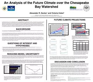
FUTURE CLIMATE PROJECTIONS ABSTRACT The purpose of this study is to analyze the projected climate over the Chesapeake Bay Watershed using the IPCC AR4 models. The A2 and B1 emission scenarios are analyzed because they bracket a business as usual emissions scenario and a more proactive emissions reduction strategy. The mean model is defined as the average of the individual models has been shown to yield the most accurate 20th century climate. By removing some poorly performing models, the mean model showed a statistically significant improvement as compared with 20th century data. With an improved mean model, it is projected that mean annual temperature will increase across the watershed by 4.65 degrees Celsius under the A2 emissions scenario and 2.49 degrees Celsius under the B1 scenario. Additionally, annual precipitation is projected to increase by 5.04% under the B1 scenario and 7.18% under the A2 scenario with the greatest increases projected for winter and spring. It is possible to speculate that changes in precipitation may alter the time and duration of the spring freshet. Flooding events and drought conditions may increase as there appears to be an upward trend in the amount of maximum 5 day rain fall, the number of consecutive dry days, and the number of extreme temperature events—particularly under the A2 scenario % B1 Precip. Anomalies Temperature Increase from Present Day An Analysis of the Future Climate over the Chesapeake Bay WatershedAlexander R. Davies1and Victoria Coles21. Department of Earth Sciences, Millersville University of PA—Millersville, PA 2. Horn Point Laboratory, University of Maryland Center for Environmental Science—Cambridge, MD. BACKGROUND This study arose out of an NSF funded Research Education for Undergraduates program run by Maryland SeaGrant in partnership with the University of Maryland Center for Environmental Science. The study took place between June and August 2007. In 1988 the World Meteorological Organization (WMO) and the United Nations Environment Programme founded the Intergovernmental Panel on Climate Change (IPCC) and gave it the task of providing reliable and non-biased information regarding climate change (IPCC, 2004). Almost twenty years after it was founded, in 2007, IPCC released the Fourth Assessment Report: “Climate Change 2007” (AR4). AR4 is an expansion upon the findings in the Third Assessment Report (TAR), released in 2001. Both the TAR and the AR4 include model assessments based on a number of scenarios. The IPCC Special Report on Emissions Scenarios (SRES) developed 40 greenhouse gas scenarios and grouped them into four “families,” A1, A2, B1, and B2, each with distinctly different directions for future developments (Nakicenovic et al., 2000). The A2 and B1 scenarios were chosen for this study. These two scenarios represent a range of emissions paths so the results will be an indication of a business as usual scenario (A2) and a proactive emissions reduction strategy (B1). The A2 scenario shows a continual and steady increase in emissions through-out the 21st century whereas the B1 scenario features a small increase in emission until mid-century followed by a decrease in emissions below current level by the end of the 21st century. Using the two scenarios highlights the effect of emissions policies on the emissions placed into the atmosphere and their impact on anthropogenic climate change over the watershed. % A2 Precip. Anomalies Figure 3 shows the A2 and B1 scenario temperature anomalies for all 12 individual models and the mean model. The anomalies are in degrees Celsius Figure 4 shows the B1 and A2 Yearly, DJF, MAM, and SON precipitation anomalies at 2025, 2050, and 2100. The anomalies are in % change and a negative sign represents a percent decrease in precipitation. Notice the % anomalies for the winter and spring months are circled. This time period is critical for the timing and duration of the spring freshet A2 Cons. Dry Days B1 Cons. Dry Days QUESTIONS OF INTEREST AND HYPOTHESIES 1. Can the uncertainty in model projections be reduced by selectively choosing models that accurately simulate the 20th Century? The hypothesis is that eliminating poorly performing models will yield a more accurate representation of the 21st Century. 2. What do the models run under different SRES scenarios suggest the physical forcing of the Chesapeake Bay watershed will be in 2025? 2050? 2100? The hypothesis is that the greatest anomalies will be seen in 2100 with anomalies being significantly smaller in 2025 and 2050. Influenced by the finding in the IPCC AR4 (IPCC, 2007), the prediction would be that air temperature will increase along with the frequency heat waves and spells, and precipitation will slightly increase with a greater frequency of heavy precipitation events. A2 Heat Wave Index B1 Heat Wave Index A2 5 Day Rain Max B1 5 Day Rain Max Table 1 shows the mean yearly, winter (DJF), and spring (MAM) snow cover anomalies the years 2025, 2050, and 2100 for the B1 and A2 emission scenarios. The anomalies are in % change and a negative sign represents a decrease in snow cover. Snow cover was calculated by multiplying the variables snc and snd for the grid points over the watershed. REDUCING MODEL UNCERTAINTY While the purpose of this study is to analyze the climate over the Chesapeake Bay watershed over the next 100 years using models and emission scenarios, first the uncertainty in the model solutions must be characterized for the region. To estimate some of the model uncertainty we use two techniques; the first is to construct a mean model to better estimate the future climate and the second is to eliminate poorly performing individual models from the mean model average. The mean model is built by averaging all the data output from all the individual models that contribute to this study. The reasoning for using the mean model is because it has been shown that on a global basis the mean model run has been the most effective at simulating 20th century climate (AchutaRao et al., 2004). To improve the mean model, we test whether eliminate poorly performing models is effective at reducing model-data error. The first step is to analyze how each individual model performs from the beginning to the end of the 20th century for a number of carefully selected variables. Raw error scores were normalized and weighted then, the final error score was calculated. The graph below on the left shows the normalized and weighted error scores. Since the mean model is constructed from the individual models, we hypothesize that removing individual model with high error scores from the mean model will improve its error score. The graph on the right shows that this is exactly what happened and in-fact , once a threshold was reached (by removing 3 models) the mean model error score began going back up suggesting that removing any more individual models reduces the accuracy of the mean model. Figure 5 shows the extreme induces (those which are calculated on a yearly basis, not a monthly). General trends were only evaluated for these variables and the mean model is represented by the black line on each graph. The top graphs are the B1 and A2 Consecutive Dry Days anomalies with anomalies in days per year. The middle graphs are for the Heat Wave Index. The anomalies are in days in which the temperature exceeds 5 degrees Celsius above the average daily temperature calculated from 1960 to 1990. The extreme temperatures must persist for a minimum of 5 days to be considered under this index. The bottom graphs are of the maximum amount of precipitation over a five day period and the anomalies are in kg/m2. DISCUSSION AND CONCLUSION The average of the IPCC AR4 ensemble is shown to have the lowest error in simulating 20th century climate, and the average can be improved by elimination of a few model outliers. The high emissions scenario projects an annual temperature increase of 4.65 degree Celsius by 2100 while the lower emissions scenario projection is 2.49 degree Celsius temperature increase. With that said, it is interesting to note the wide range of individual model projections as seen in Figure 3. The model projecting the lowest temperature anomaly is the GISS-ER under the B1 scenario. It projects a 1.62 degree Celsius annual increase in temperatures while the MIRCO3.2-medres under A2 conditions projects a 6.16 degree Celsius increase. This represents a 4.54 degree Celsius range of variability which illustrates the uncertainty and variability in the projections of regional climate change. Precipitation is important to the region because its implications for water supply and agriculture; however here we consider its effect on stream flow. While there is only a weak correlation between precipitation and stream flow, the literature suggests enough of a relationship between the two that precipitation can give a rough idea as to the amount of stream flow entering the bay. When assessing the fresh water influx into the bay, a critical time is during the spring freshet. The Chesapeake Bay usually receives a peak in fresh water influx roughly around the beginning of April. From Figure 4 it would be reasonable to speculate that the spring freshet might come sooner in the year due to the increases in precipitation in not only spring, but also winter. Also because of the general increase in precipitation in both winter and spring, it may also be reasonable to speculate that the freshet will be more gradual instead of having a pronounced peak at some point in the year. The results shown in Table 1 are also critical for the freshet however a full hydrologic model is need to gain a full understanding. The conclusion to be made here is that we have a choice. The A2 scenario represents a world where little is done to retard the amount of emissions placed into the atmosphere. The B1 scenario represents a world where policy changes take place and emissions decrease. As a result, the 2100 projections under the B1 scenario are not as extreme or severe as those under the A2 scenario. Now is the time to make the choice as a global society as to which path we will take. Normalized and Weighted Error Mean Model Acknowledgments: David Kimmel (UMCES) Maryland Sea Grant REU Program Horn Point Laboratory, University of Maryland Center for Environmental Science National Science Foundation Sepi Yalda and Richard Clark (MU), Ander Muller (USNA) MDSG REUs Class of 2007 We acknowledge the modeling groups, the Program for Climate Model Diagnosis and Intercomparison (PCMDI) and the WCRP's Working Group on Coupled Modeling (WGCM) for their roles in making available the WCRP CMIP3 multi-model dataset. Support of this dataset is provided by the Office of Science, U.S. Department of Energy Figure 1 shows the normalized weighted scores each individual model got along with the control score for the mean model that includes all 15 individual models. As a reminder, the best possible score is zero and the worst possible score is 14. The models used in the project are along the left hand side and the colors correspond with the error bars on the graph. Figure 2 shows how the error associated with the mean model changed as individual models were removed from the mean model. The models were removed in the order based upon their error scores as shown in Figure 1 to the left. Works Cited: AchutaRao K, Covey C, Doutriaux C, Fiorino M, Gleckler P, Phillips T, Sperber K, and Taylor K. 2004. An Appraisal of Coupled Climate Model Simulations. U.S. Department of Energy and University of California, Lawrence Livermore National Laboratory. Contract W-7405-Eng-48 Intergovernmental Panel on Climate Change (IPCC). 2004 Dec [cited 2007 June 5]. 16 Year of Scientific Assessment in Support of the Climate Convention. Available from: http://www.ipcc.ch/about/anniversarybrochure.pdf Nakicenovic N, Alcamo J, Davis G, de Vries B, Fenhann J, Gaffin S, Gregory K, Grübler A, Jung TY, Kram T, Lebre La Rovere E, Michaelis L, Mori S, Morita T, Pepper W, Pitcher H, Price L, Riahi K, Roehrl A, Rogner H, Sankovski A, Schlesinger M, Shukla P, Smith S, Swart R, Van Rooijen S, Victor N and Dadi Z. 2000 [cited 2007 June 5]. Intergovernmental Panel on Climate Change: Special Report on Emissions Scenarios. Available from: http://www.grida.no/climate/ipcc/emission/


