Download
1 / 38
380 likes | 688 Views
Three Types of Design Structures Completely Randomized/Factorial Designs……………… p. 3 Block Designs…………………… ……….....…… …………... p. 6 Split Plot/Repeated Measures Designs ……………..…… p. 9 Crossed vs. Nested Factors ……………..…..…. p. 11 Mathematical Calculations ……………..………… p. 21

E N D
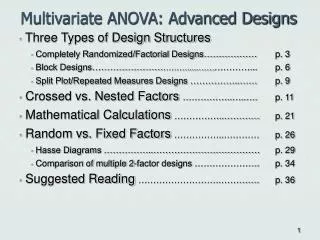
Three Types of Design Structures • Completely Randomized/Factorial Designs……………… p. 3 • Block Designs…………………………….....………………... p. 6 • Split Plot/Repeated Measures Designs ……………..…… p. 9 • Crossed vs. Nested Factors ……………..…..…. p. 11 • Mathematical Calculations ……………..………… p. 21 • Random vs. Fixed Factors ……………..………… p. 26 • Hasse Diagrams ……………..……………………………… p. 29 • Comparison of multiple 2-factor designs …………………. p. 34 • Suggested Reading ……………………….…………. p. 36 Multivariate ANOVA: Advanced Designs
Multivariate ANOVA: Advanced Designs • The previous section introduced Analysis of Variance (ANOVA) by discussing one type of design structure, the randomized basic factorial design. This presentation will provide a general introduction to complex design structures. In order to appropriately analyze an experiment, it is necessary to answer the following questions: • Is structure of the design: • a Complete Randomized Design (CR) also called the Randomized Basic Factorial Design or Factorial Design • a Block Design, or • a Split Plot/Repeated Measure Design • 2) Is each factor crossed or nested. • Is each factor fixed or random. • The F test in all ANOVAs are based on comparing factor variability and residual variability (i.e. MSA/MSE).The answers to these three questions are necessary in order to 1) understand variability, 2) develop appropriate ANOVA models, and 3) drawing conclusions from any study.
18 E.U 3 treatments Plain Aspirin Floral Compound 18 E.U Randomly assign a treatment to each flower Three Types of Design Structures In Completely Randomized/Factorial Designs, each condition (specific combination of factor levels) is randomly assigned to an Experimental Unit (EU). There are no restrictions on how conditions are assigned to Experiment Units. EXAMPLE 1: Students in an introductory statistics class tested the impact of additives on the longevity of cut flowers. They purchased 18 carnations and randomly assigned one of three treatments (plain water, one aspirin added to the water, and a floral compound provided by the flower shop) to each flower. Factor: water additive with Levels: plain, aspirin, and floral compound Unit or EU (experimental unit): each of the 18 flowers Response: longevity (i.e. number of days until flower starts to wilt) Null hypothesis: additives make no difference in the longevity of carnations.
Three Types of Design Structures • This study could be analyzed with a 1-factor ANOVA, with factor A, Additive, having three levels. An F statistic would be used to determine if the variability between the level means of factor A, MSA, is large compared to the general flower to flower variability, MSE. Before the students can determine if the results of their study extent to the general population of all carnations, they need to also address other issues: • What care did they take in the experimental process to ensure that other external factors did not influence the longevity? For example, were the carnations stems cut at the same time and in the same way? Were the carnations exposed to the same amount of sunlight, temperature, and humidity levels? • Is there sample truly representative of the the entire population? If their sample was all the same color or from the same store it is very likely that the MSE they calculate from their sample will show less variability than a true random sample from the entire population. If the MSE is not accurate, the ANOVA is not valid. • In order to draw conclusions from any experiment, is essential to realize that the experiments design and procedures are just as important (if not more important) than any statistical calculations.
Three Types of Design Structures To address these issues, it is important to write very clear procedures before the experiment begins. For example, since flowers absorb moisture through the stem, the angle at which a stem is cut is known to impact flower longevity. Unless cut angle is another variable in their experimental design, it is important that this potential nuisance variable is kept as consistent as possible. These students also chose to restrict their experiment to only white carnations. Since it is impossible to select a true random sample from all carnations sold on a particular date, the students had purchased 6 white carnations from three different stores. While not perfect, this is a very practical approach to account for population variability of white carnations. Store type clearly was not a factor of interest, but it could impact the results. Thus it is fitting to include the nuisance factor, Store, in the model and analyze the data using a Randomized Block Design ANOVA instead of a Completely Randomized ANOVA.
Three Types of Design Structures In factorial designs, a treatment is a specific combination of predetermined factor levels that is assigned to an EU. However there are many situations in which a study also includes nuisance factors (factors that may impact the results but not be of specific interest in the study). Blocking incorporates nuisance factors into the design in order to provide more accurate results. Blocking is the process of grouping units based on some pre-existing similarity that might impact the results. Units can be sorted, reused, or subdivided to create a block. Block effects can be of interest in a study, however since blocks are pre-existing conditions and thus not assigned to EU, there is no causation. Even without proving causation, blocking is extremely useful if it can explain some of the model variability. The Mathematical Calculations section will describe that including the blocking factor may reduce the experimental error (MSE) and thus help identify other factors of interest as significant.
Store 1 6 E.U Store 2 6 E.U Store 3 6 E.U Store 1 6 E.U Store 2 6 E.U Store 3 6 E.U 3 treatments Plain Aspirin Floral Compound Within each block (store) randomly assign a treatment to each flower Three Types of Design Structures Block Designs restrict the way in which the conditions are assigned. Units are placed into groups (or blocks) of similar units. Units within each group are assumed to have some similarity that may impact the results . Within each block, treatments are randomly assigned to one unit. EXAMPLE 1 (continued): The random assignment of treatments to units was done within each block. Since there are an equal number of treatments for each store, the effect of additive is not biased by store type. In addition, the students are able to measure the variability that exists between stores. *The Mathematical Calculations section will explain that while this is a block design, the ANOVA is identical to a 2-factor ANOVA with no interaction term. One F-test for store effect and another for additive effect.
18 E.U Store 1 6 E.U Store 2 6 E.U Store 3 6 E.U Store 1 6 E.U Store 2 6 E.U Store 3 6 E.U 3 treatments Plain Aspirin Floral Compound Within each block (store) randomly assign a treatment to each flower Three Types of Design Structures Before the third design structure is discussed, it is important to understand the difference between replications and repeated measures. Replications occur when each condition is assigned to more than one unit. In the factorial design in Example 1, each condition had 6 replicates (6 flowers units) that was assigned to each level of the Additive factor. In the block design in Example 1, each condition had 2 replicates (2 flower units) assigned to each level within each block. 3 treatments Plain Aspirin Floral Compound 18 E.U Randomly assign a treatment to each flower Repeated Measuresoccur when multiple conditions are assigned to one unit. Thus replications have one measurement for each unit while repeated measurements have multiple measurements on one unit.
3 Boxes of Brand A Popcorn 3 Boxes of Brand A Popcorn 3 treatments Refrigerator Room temperature 3 Boxes of Brand B Popcorn 3 Boxes of Brand B Popcorn Randomly select 2 bags within each box Three Types of Design Structures Split Plot/Repeated Measures Designs have two sizes of units in one design. A condition is assigned to a whole plot unit and then the whole plot unit is reused or subdivided into subgroups (split plot units) which also receive a condition. The whole plot units act as blocks for the split plot units. EXAMPLE 2: To test the effect of storage temperature and brand on the percentage of popped kernels, a student purchased three boxes of both an expensive (exp) and generic (gen) popcorn brand. Each box contained six microwavable bags. Two bags were randomly selected from each box and stored for one week, one in the refrigerator (frig) and the other at room (room) temperature. The bags were popped in random order and the popped and un-popped kernels were counted.
Three Types of Design Structures Whole Plot Factor: brand Whole Plot Unit (Blocks): Box Split Plot Factor: storage temperature Split Plot Unit: Bag Response: % popped kernels in a bag The popcorn bags within a box is considered a repeated measure (not a replicate) when testing Brand because the bag to bag variability with a Box is not representative of the population variability. The Bags within each Box are likely to be handled by the same operator, at the same time and at the same location. Since Boxes were randomly selected from each brand population, they are replicates and a better measure of the experimental error (whole plot MSE) within brands. The Bags within a Box are considered as sub plot units. To test the effect of storage temperature, Bags were randomly assigned to a treatment (frig or room) so Bags are the appropriate experimental error (split plot MSE) to measure the temperature effect.
Factors A and B are crossed if every level of A can occur in every level of B. Factor B is nested in factor A if levels of B only have meaning within specific levels of A. In Factorial Designs all factors of interest are crossed and there are no repeated measures. Block Designs can have either crossed or nested factors. Units are always nested within blocks. EXAMPLE 1: Store and additive are crossed factors, since the same additive is assigned to flowers from each store. The additive effects (treatments 1, 2, and 3) have meaning across storesand each store effect can also be calculated. Six flowers (units) are nested within each of the three stores. The first white carnation purchased from Store 1 is not expected to have any relation to the first flower purchased from Store 2. So finding a Flower 1 effect is meaningless. If three red flowers and three white flowers were purchased within each store, then flower color would be crossed with store, even though flowers (units) are still nested within each store. *This would be a 2-way block design, since 2 factors of interest (color and additive) are in each block. Crossed Vs. Nested Effects
Split Plot Designs typically have both crossed and nested effects. EXAMPLE 2: The whole plot unit (Boxes) are nested in Brand. The three Boxes (B1, B2, B3) appear only under the expensive level of factor A (Brand) and the next three boxes (B4, B5, B6) appear only under the generic level of factor A. In many texts, B4 ,B5, and B6 are also labeled B1 ,B3, and B3, but it is understood that the B1 occurring in expensive is different from the B1 occurring in generic. Bags are nested within Boxes. Each Bag can only come from one Box. Also remember that units are nested in blocks. Storage Temperatures are crossed with Brand. Each Temp occurs in each Brand [room (T1) and frig (T2) occur in each Brand]. Since these factors are crossed, room (T1) is the same under both the expensive and the generic Brands. Storage Temperatures are also crossed with Box, but this interaction effect is of no interest and typically not shown in an ANOVA table. Crossed Vs. Nested Effects
The calculations for effect size depends on whether a factor is crossed or nested. The effect calculations do not depend on whether the factor is a factor of interest or a nuisance factor (block). As shown in the Factorial Design tutorial, all crossed effects are calculated by finding the appropriate average and subtracting the partial fit. All nested effects are also calculated by finding the appropriate average and subtracting the partial fit. However, partial fits in nested factors includes the factor level in which it is nested. EXAMPLE 1: The effect of “aspirin additive” is the average result of all flowers treated with the aspirin additive minus the Grand Mean. The “store 3” effect is the average result of all flowers purchased from store 3 minus the grand average. EXAMPLE 1: Flower (unit) is nested within Store. The effect of the 1st flower from Store1 is calculated: (Average of flower 1 within Store1) - (Store1 effect + Grand Mean) Note that the flower effect is used to calculate MSE. In this study each flower is the unit and the average is just the observed result for that flower. Calculating Crossed Vs. Nested Effects
Grand Mean Brand Temp Box Brand*Temp Bag EXAMPLE 2: We can visualize the design structure of any balanced model with a Hasse diagram, which lists each factor. Interaction terms are listed below the main effects and arrow point from the interaction to the main effects. Arrows also point from nested factors to the factors in which they are nested. Calculating Crossed Vs. Nested Effects Temperatures and brand are crossed: only the Grand Mean is included in their partial fit. Boxes are nested in Brand: Brand and Grand Mean are included in their partial fit. The Brand by Temp interaction includes both Brand and Temp. Thus the partial fit for this term includes the Brand, Temp and Grand Mean effects. Bags are nested within Boxes (and so also is necessarily nested within Brand). Bags are also randomly selected within Temp. The partial fit for Bag includes the Box, Brand, Brand*Temp, Temp and Grand Mean effects.
The tables show a slightly modified data set for Example 2. Main effects for crossed factors are found by subtracting the Grand Mean from the appropriate averages. Calculating Crossed Vs. Nested Effects Grand Mean = 84
The Main Effects plot shows that the effect of Brand is larger than the effect of Temp. In this sample, the Expensive Brand did better than Generic and Refrigerated bags did better than Room Temperature bags. Calculating Crossed Vs. Nested Effects Even though the graph appears to show a difference between levels, we do not know at this time whether these differences are significant. In other words, if there really is no difference in Brand, how often would we expect effects this large in a random sample?
The Brand by Temp interaction is also found with the following formula: Level Average - (Brand effect + Temp effect + Grand Mean). Calculating Crossed Vs. Nested Effects
Referring back to the Hasse diagram, we still need to calculate the effects of Box and Bag.Since each Box only has meaning within a Brand, there are 6 box averages that need to be calculated Calculating Crossed Vs. Nested Effects Crossed effects always sum to zero. Nested effects (Box) also sum to zerowithin each appropriate factor level (Brand). Box B1, B2, and B3 effects sum to zero within the exp Brand. Box B1, B2, and B3 effects sum to zero within the gen Brand.
Since Bags are the units in this study, the Bag effect is the same as a residual effect. To calculate the residual effect, subtract all other effects from the Bag average (observed % popped from each bag). Crossed Vs. Nested Effects Effect sizes still sum to 0
Grand Mean Brand Temp Box Brand*Temp Bag • In Summary: • All effect sizes are calculated by finding the appropriate average and subtracting the partial fit. • Partial fits depends on whether a factors are crossed or nested. • Hasse diagrams are helpful in visualizing complex design structures. Calculating Crossed Vs. Nested Effects
Effects show the impact of each factor combination and identify which factors are most influential in our sample. However, a statistical hypotheses test is needed in order to determine if any of these effects are significant. Each row corresponding to a factor of interest in the Analysis of variance (ANOVA) consists of hypothesis tests to determine if there is statistical evidence that the effects are non-zero. While effect size calculations vary depending on whether the factor is crossed or nested, the following calculations are used for all terms in all balanced designs: Sum of Squares (SS) = sum of all the squared effects Degrees of Freedom (df) = number of free units of information Mean Square (MS) = SS/df for each factor In some designs, there are multiple unit sizes and each unit size has an experimental error (residual) term. The appropriate denominator (MSE) in the F tests will depend on the three initial questions: 1) design structure, 2) crossed vs. nested factors, and 3) fixed vs. random factors. Mean Square Error (MSE) = pooled variance of samples within each level F statistic = MS for each factor/MSE Mathematical Calculations
Sum of Squares (SS) is calculated by summing the squared factor effect for each run, . For Example 2: Mathematical Calculations Sum of Squares
Degrees of Freedom (df) = number of free units of information. In Example 2), there are 2 levels of Brand and the ANOVA assumptions require that the effects sum to 0. Knowing the effect of the generic brand, automatically forces a known expensive brand effect. a = # of levels in Brand, b = # of levels in Temp, c = # of levels of Bags within each Brand Mathematical Calculations For factors not nested in any other factors,the df is the number of levels minus one. dfBrand = dfA = a – 1 = 2-1 = 1 dfTemp = dfB = b – 1 = 2-1 = 1 For nested factors, restrictions in ANOVA require that all nested effects sum to zerowithin each level of the factor it is nested in. Box, factor C, is nested in Brand. The three boxes in the Expensive brand need to sum to 0. If two effects in expensive are known, the third box effect is fixed. There are c-1 pieces of free information for every level of Brand. dfBox = dfC = a * (c – 1) = 2(3-1) = 4
For the Brand*Temp (AB) factor interaction there are a*b effects that are calculated. Restrictions in ANOVA require Mathematical Calculations • AB interaction factor effects sum to 0. This requires 1 piece of information to be fixed. • The interaction effects within the exp Brand level sum to 0. The same is true for the gen Brand level. This requires 1 piece of information to be fixed in each Brand level. Since 1 value is already used in restriction 1), this requires a-1 pieces of information. • The AB effects also sum to 0 within each Temp level. This requires b-1 pieces of information. • Thus, general rules for a factorial ANOVA: • dfBrand*Temp= dfAB = ab – [(a-1) + (b-1) + 1] = (a-1)(b-1) • = 4 – [1+1+1] =1 Similarly, the df for residuals (bags in our example) also fits these restrictions. dfBag = # of effects – [pieces of information already accounted for] = # of effects – [dfBox + dfAB + dfBrand + dfTemp + 1] = abc – [a(c-1) + (a-1)(b-1) + (a-1) + (b-1) + 1] = 12 – [2(3-1) + (2-1)*(2-1) + (2-1) + (2-1) +1] = 4 where abc = number of units (cups)
Mean Squares (MS) = SS/df for each factor. MS is a measure of variability for each factor. Below is the ANOVA for Example 2): Source DF SS MS F P Brand 1 3.00 3.00 0.18 0.697 Box(Brand) 4 99.00 24.75 1.45 0.364 Temp 1 1.33 1.33 0.08 0.794 Brand*Temp 1 96.33 96.33 5.64 0.076 Error 4 68.33 17.08 Total 11 268.00 F statistic = MS for each factor/MSE. Since there are 2 unit sizes, Boxes and Bags, there are two error (MSE) terms. The Brand F ratio uses Box(Brand) [stated Box nested within Brand] in the denominator. Since Box best represents the variation within Brand, it is the whole plot error. To test the effect of temperature, we have two bags that are as similar as possible (i.e. from the same Box) and randomly assign each Bag to either room or frig. The F ratio for Temp is MSTemp/MSBag.MSBag = MSE and is called the split plot error. In addition to the design structure and crossed vs. nested factors, each factor needs to be classified as fixed or random in order to determine what error term should be used in the denominator for every F test. Mathematical Calculations
Fixed factors: the levels tested represent all levels of interest Random factors: the levels tested represent a random sample from some population of possible levels of interest. EXAMPLE 1: The levels of water Additive, (plain, aspirin, and floral compound) are all of specific interest. They are not just a random selection of all possible items that could be added to water. Thus, Additive is a fixed factor. The students did not want to compare three specific stores to determine which store had the best flowers. Instead three stores were selected to better understand the variability that exists within the population. Store and Flowers (units) are random factors. EXAMPLE 2: Bags and Boxes are random factors. There were random selections from a population of Boxes and a population of Bags. Brand and Temp are fixed factors. If we were not interested in finding the effect of exp and gen Brands, but instead simply randomly selected two types of Brands from all possible Brands, then Brand would be a random factor.Determination of whether effects are fixed or random can vary, and the choice can greatly impact the ANOVA analysis. There are some general rules to determine whether a factor is fixed or random. Fixed Vs. Random Effects
Fixed Vs. Random Effects Fixed factors have meaning only at the levels that were included in the experimental design. The same levels of that factor would be used if the experiment was repeated. Since the levels of random factors were randomly selected, the results have meaning for the levels selected in the study as well as any levels not included in the study. Different levels would be randomly selected if the experiment was repeated. Blocks and units are typically classified as random effects. • Now that the key questions have been answered: • Is structure of the design: • a Complete Randomized Design/Factorial Design • a Block Design, or • a Split Plot/Repeated Measure Design • 2) Is each factor is crossed or nested. • Is each factor is fixed or random. • Hasse diagrams can be used for to determine what error term should be used in the denominator for every F test. Hasse diagrams are effective for all balanced designs (same number of units in every condition).
1) Start row 1 with node M for the grand mean 2) Put a node on row 2 for each factor that is not nested in any term. Add arrows from each node on row 2 to the grand mean. Place parentheses around any random factor. 3) Add a node on row 3 for any factor nested in row 2, and draw arrows to the row 2 nodes. Add a node for any 2-way interaction and draw arrows to the individual factors in row 2. Place parentheses around any random factor or any factor that is nested in a random factor. If an interaction term contains at least 1 random effect, the entire interaction is considered random. 4) On each successive row, say row “i”, add a node for any factor nesting in row “i-1”. Add a node for any “i-way interaction”. Draw appropriate arrows to the “i-1” nodes and place parentheses around any random factor or any factor that is nested in a random factor. 5) When all interactions or nested factors are exhausted, add a node for error on the bottom line, and draw arrows to nodes in the row above. 6) For each node, add a superscript that indicates the number of effects for each term. (# of interaction effects are always products of the # of main effects) 7) For each node, add a subscript that indicates the degrees of freedom for that term. Degrees of freedom for a term are found by starting with the superscript for that particular node and subtracting out the degrees of freedom for all terms connected with arrows above it. Rules for Developing Hasse Diagrams
If the Hasse Diagram is developed, the denominator for the appropriate F test is typically straightforward: The denominator for testing node A is the next eligible random term below A in the Hasse diagram. If there are 2 or more “next eligible random terms” then use an approximate test. Approximate tests usually are a combination of existing MS values. Most software packages do this automatically. In more complex models that included mixed interaction terms (there are both fixed and random factors in the interaction), it is necessary to determine whether the effects are Restricted or Unrestricted. In general restricted effects sum to zero while unrestricted effects do not. However, this classification tends to be rather complex and the analysis is best done with a statistician. Texts listed at the end of this tutorial all discuss the restricted and unrestricted effects in more detail. Mathematical Calculations: Hasse Diagram
Store 1 6 E.U Store 2 6 E.U Store 3 6 E.U Store 1 6 E.U Store 2 6 E.U Store 3 6 E.U 3 treatments Plain Aspirin Floral Compound Within each block (store) randomly assign a treatment to each flower Hasse Diagram for Example 1) Mathematical Calculations 1) Start row 1 with a node for the grand mean 2) Put a node on row 2 for each factor that is not nested in any term. Add arrows from each node on row 2 to the grand mean. Place parentheses around any random factor. 3) Add a node on row 3 for any factor nested in row 2, and draw arrows to the row 2 nodes. Place parentheses around any random factor or any factor that is nested in a random factor. No 2-factor interactions are used. 4) No successive rows needed. Grand Mean (Store) Additive (Flower)
Hasse Diagram for Example 1 (continued): Mathematical Calculations • 5) When all interactions or nested factors are exhausted, add a node for error on the bottom line, and draw arrows to nodes in the row above. • 6) For each node, add a superscript that indicates the number of levels for each term. (# of interaction effects are always products of the # of main effects) • For each node, add a subscript that indicates the degrees of freedom for that term. Degrees of freedom for a term are found by starting with the superscript for that particular node and subtracting out the degrees of freedom for all terms connected with arrows above it. Grand Mean11 (Store)32 Additive32 (Error) 1813 Flowers are the units, thus the flower effect is identical to the residual effect (i.e. the error term). For this study, there is only one error term (thus only one MSE). Error is the first random term following the Store effect and the Additive effect. Thus error (i.e. flower or unit) is the denominator in both F tests.
Grand Mean Brand Temp (Box) Brand*Temp (Bag) Hasse Diagram for Example 2): 1) Start row 1 with a node for the grand mean 2) Put a node on row 2 for each factor that is not nested in any term. Add arrows from each node on row 2 to the grand mean. 3) Add a node on row 3 for any factor nested in row 2, and draw arrows to the row 2 nodes. Add a node for any 2-way interaction and draw arrows to the individual factors in row 2. Place parentheses around any random factor or any factor that is nested in a random factor. If an interaction term contains at least 1 random effect, the entire interaction is considered random. 4) On each successive row, say row “i”, add a node for any factor nesting in row “i-1”. Add a node for any “i-way interaction”. Draw appropriate arrows to the “i-1” nodes and place parentheses around any random factor or any factor that is nested in a random factor. Mathematical Calculations
Grand Mean11 Brand21 Temp21 (Box)64 Brand*Temp41 (Error) 124 Hasse Diagram for Example 2: Mathematical Calculations • 5) When all interactions or nested factors are exhausted, add a node for error on the bottom line, and draw arrows to nodes in the row above. • 6) For each node, add a superscript that indicates the number of levels for each term. (# of interaction effects are always products of the # of main effects) • For each node, add a subscript that indicates the degrees of freedom for that term. Degrees of freedom for a term are found by starting with the superscript for that particular node and subtracting out the degrees of freedom for all terms connected with arrows above it. For this study, Box (whole plot error) is used in the denominator for the F test for the effect of Brand. Bag (Error or sub plot error) is the first random term below Temp and Brand*Temp, thus error (i.e. bag or split plot unit) is the denominator in both Temp and Brand*Temp F tests.
Comparison of 2 factor models: The following ANOVA tables use identical data. However, each ANOVA calculation is different because it is based on different assumptions. Create Hasse diagrams for the following 4 designs to verify if the appropriate error terms were used. A and B crossed [written A x B or AB], any combination of fixed and random effects. Source df SS MS F p B 1 1200 1200 33.33 0.00 A 2 2600 1300 36.11 0.00 Error 8 288 36 Total 11 4088 A nested in B [this is written A(B)], A fixed B fixed: Source df SS MS F p B 1 1200 1200 52.94 0.00 A(B) 4 2752 688 30.35 0.00 Error 6 136 22.67 Total 11 4088 Effect Classifications in 2-way ANOVA
Comparison of 2 factor models: The following ANOVA tables use identical data. However, each ANOVA calculation is based on different assumptions. A nested in B [this is written A(B)], A random B fixed: Source df SS MS F p B 1 1200 1200 1.74 0.26 A(B) 4 2752 688 30.35 0.00 Error 6 136 22.67 Total 11 4088 A nested in B [this is written A(B)], A random B random: Source df SS MS F p B 1 1200 1200 1.74 0.26 A(B) 4 2752 688 30.35 0.00 Error 6 136 22.67 Total 11 4088 *It typically doesn’t make sense to have a fixed factor nested within a random factor. For example, it you randomly select 10 trees, factor B, and then choose 5 leaves nested within each tree, factor A. It is reasonable since trees are random, so are the trees. Effect Classifications in 2-way ANOVA
Suggested Reading • Hunter, W. G., “Some Ideas about Teaching and Design of Experiments, with 2^5 Examples of Experiments Conducted by Students”, The American Statistician, Vol. 31, No. 1 (Feb., 1977), 12-17. • Suggested Textbooks • Design and Analysis of Experiments by George Cobb, • Prerequisites: none • Examples: wide variety • Design and Analysis of Experiments by Gary Oehlert, • Prerequisites: prior statistics courses are beneficial • Examples: primarily from science and engineering • Design and Analysis of Experiments by Davig Montgomery, • Prerequisites: prior statistics courses are beneficial • Examples: primarily engineering
Suggested Reading • The structure, or Hasse, diagram described by Taylor and Hilton (American Statistician, 1981) provides a visual display of the relationships between factors for balanced complete experimental designs. Using the Hasse diagram, rules exist for determining the appropriate linear model, ANOVA table, expected means squares, and F-tests in the case of balanced designs. • Kempthorne, O. (1982). Classificatory Data Structures and Associated Linear Models, • in Essays in Honor of C. R. Rao, G. Killianpur, P. R. Krishnaiah, J. K. Ghosh,eds. New York: North Holland, 397-410. • Lohr, S. L. (1995). Hasse Diagrams in Statistical Consulting and Teaching. The American Statistician, 49, 4, 376-381. • Marasinghe, M. G. and Darius P. L. (1990). A Structure-based Approach for Model Determination in Experimental Designs. Proc. Stat. Comp. Section, American Statistical Association, 143-150. • Oehlert, G., “A First Course in Design and Analysis of Experiments”, Freeman Publishers, 2000 • Searle, S. R. (1971). Linear Models. New York: Wiley. • Taylor, W. H. and Hilton, H. G. (1981). A Structure Diagram Symbolization for Analysis of Variance. The American Statistican, 35, 2, 85-93. • http://www.jstatsoft.org/v13/i03/v13i03.pdf
The following are addition terms and techniques that can be used in developing advanced ANOVA models. While many of these are beyond the scope of this tutorial, they are all discussed in more detail in the suggested textbooks: Often factors or designs are described based of their relationship to units. When units are nested within factors, they are called between group factors. If some combination of factors are allocated within units, they are called within group factors. Latin Square Designs are designs with two blocking factors (two nuisance factors) and one factor of interest. Nested designs are also called hierarchical designs. These designs can have 3 or more levels of nesting. For example, trees could be nested within fields and leaves nested in trees. Additional Terminology