Exploring Assumptions
Exploring Assumptions. Chapter 5. Assumptions of Parametric Data. Parametric tests are based on the normal distributions and the following must be met: Normally distributed data. Homogeneity of variance: Variances should be equal throughout the data The groups should have equal variance

Exploring Assumptions
E N D
Presentation Transcript
Exploring Assumptions Chapter 5
Assumptions of Parametric Data • Parametric tests are based on the normal distributions and the following must be met: • Normally distributed data. • Homogeneity of variance: • Variances should be equal throughout the data • The groups should have equal variance • In corr: the variance in one variable (x) should be equal across all levels of the other variable (y). • Dependent variable should be interval or ratio. • Independence: for independent designs the data from different subjects should be independent; for repeated designs the time variable will be dependent, but different subjects should be independent.
Assumption of Normality • Many statistical tests (t, ANOVA) assume that the sampling distribution is normally distributed. • This is a problem, we don’t have access to the sampling distribution. • But, according to the central limit theorem if the sample data are approximately normal, then the sampling distribution will be normal. • Also from the central limit theorem, in large samples (n > 30) the sampling distribution tends to be normal, regardless of the shape of the data in our sample.
Explore Command In SPSS, use: Analyze – Descriptives – Explore to get to the Explore Command.
The P-P Plots is a probability-probability plot. From the Explore command it compares the variables cumulative probability to the cumulative probability of the normal distribution. If the circles fall on the line the data are normal. Day 2 & Day 3 are NOT normal. It is clear from the histograms that they are both positively skewed.
Interpretation of Deviations of Skew and Kurtosis based on Z Scores Z > 1.95 is significant at p < .05 Z > 2.58 is significant at p < .01 Z > 3.29 is significant at p < .001 Day 1 is platykurtic (flat), Days 2 & 3 are leptokurtic (peaked)
Interpretation of Deviations of Skew and Kurtosis based on Z Scores Z > 1.95 is significant at p < .05 Z > 2.58 is significant at p < .01 Z > 3.29 is significant at p < .001 Day 1 is platykurtic (flat), Days 2 & 3 are leptokurtic (peaked)
Interpretation of Deviations of Skew and Kurtosis based on Z Scores Z > 1.95 is significant at p < .05 Z > 2.58 is significant at p < .01 Z > 3.29 is significant at p < .001 Day 1 is platykurtic (flat), Days 2 & 3 are leptokurtic (peaked)
Large Samples and Z Scores Z > 1.95 is significant at p < .05 Z > 2.58 is significant at p < .01 Z > 3.29 is significant at p < .001 • Significance tests of skew and kurtosis should not be used in large samples (because they are likely to be significant even when skew and kurtosis are not too different from normal.
With the combined groups (Duncetown & Sussex) Numeracy looks positively skewed.
You can split a file by groups (as in the next 2 slides) or just use existing groups and add the grouping variable to the factor list.
Just as in the p-p Plot, the Q-Q Plot the data should fall on the line if the data set is normal. Both of these variables have a problem with Normality.
The plot on the left shows unequal variance. This would be evident when looking at: sd’s, variance and the Levine’s Test of Homogeneity of Variance.
Numeracy from SPSSExam.sav Variance Duncetown University 4.271 Sussex University 9.432 N = 50
Outliers and Extreme Scores KINE 5305 Applied Statistics in Kinesiology
SPSS – Explore BoxPlot • The top of the box is the upper fourth or 75th percentile. • The bottom of the box is the lower fourth or 25th percentile. • 50 % of the scores fall within the box or interquartile range. • The horizontal line is the median. • The ends of the whiskers represent the largest and smallest values that are not outliers. • An outlier, O, is defined as a value that is smaller (or larger) than 1.5 box-lengths. • An extreme value, E , is defined as a value that is smaller (or larger) than 3 box-lengths. • Normally distributed scores typically have whiskers that are about the same length and the box is typically smaller than the whiskers.
Check your data to verify all numbers are entered correctly. Verify your devices (data testing machines) are working within manufacturer specifications. Use Non-parametric statistics, they don’t require a normal distribution. Develop a criteria to use to label outliers and remove them from the data set. You must report these in your methods section. If you remove outliers consider including a statistical analysis of the results with and without the outlier(s). In other words, report both, see Stevens (1990) Detecting outliers. Do a log transformation. If you data have negative numbers you must shift the numbers to the positive scale (eg. add 20 to each). Try a natural log transformation first in SPSS use LN(). Try a log base 10 transformation, in SPSS use LG10(). Decisions for Extremes and Outliers
Add 10 to the data. Then log transform. Add 10 to each data point. Try Natural Log. Last option, use Log10.
Add 10 to each data point, since you can not take a log of a negative number.
Outlier Criteria: 1.5 * Interquartile Range from the Median Milner CE, Ferber R, Pollard CD, Hamill J, Davis IS. Biomechanical Factors Associated with Tibial Stress Fracture in Female Runners. Med Sci Sport Exer. 38(2):323-328, 2006. Statistical analysis. Boxplots were used to identify outliers, defined as values >1.5 times the interquartile range away from the median. Identified outliers were removed from the data before statistical analysis of the differences between groups. A total of six data points fell outside this defined range and were removed as follows: two from the RTSF group for BALR, one from the CTRL group for ASTIF, one from each group for KSTIF, and one from the CTRL group for TIBAMI.
Outlier Criteria: 1.5 * Interquartile Range from the Median (using SPSS)
Outlier Criteria: 1.5 * Interquartile Range from the Median (using SPSS) Outliers = 1.5 * 3.39 above and below -.3549
Outlier Criteria: ± 3 standard deviations from the mean Tremblay MS, Barnes JD, Copeland JL, Esliger DW. Conquering Childhood Inactivity: Is the Answer in the Past? Med Sci Sport Exer. 37(7):1187-1194, 2005. Data analyses. The normality of the data was assessed by calculating skewness and kurtosis statistics. The data were considered within the limits of a normal distribution if the dividend of the skewness and kurtosis statistics and their respective standard errors did not exceed ± 2.0. If the data for a given variable were not normally distributed, one of two steps was taken: either a log transformation (base 10) was performed or the outliers were identified (± 3 standard deviations from the mean) and removed. Log transformations were performed for push-ups and minutes of vigorous physical activity per day. Outliers were removed from the data for the following variables: sitting height, body mass index (BMI), handgrip strength, and activity counts per minute.
Computing and Saving Z Scores Check this box and SPSS creates and saves the z scores for all selected variables. The z scores in this case will be named zLight1…
Computing and Saving Z Scores Now, you can identify and remove raw scores above and below 3 sds if you want to remove outliers.
Comparison of Outlier MethodsMedian ± 1.5 * Interquartile Range27 ± 1.5 * 7 gives a range of 16.5 – 37.5
Comparison of Outlier Methods± 2 SDs (Notice the 16s are not removed)
Comparison of Outlier Methods± 2 SDs (Notice the 16s are not removed)
Comparison of Outlier Methods± 3 SDs (Step 1, then run Z scores again)
Comparison of Outlier Methods± 3 SDs (Step 2, after already removing the -44, the -2 then has a SD of -4.68 so it is removed)
The median ± 1.5 * interquartile range appears to be too liberal. ± 2 SDs may also be too liberal and statisticians may not approve. An iterative process where you remove points above and below 3 SDs and then re-check the distribution may be the most conservative and acceptable method. Choosing 3.1, 3.2, or 3.3 as a SD increases the protection against removing a score that is potentially valid and should be retained. Conclusions?
Check your data to verify all numbers are entered correctly. Verify your devices (data testing machines) are working within manufacturer specifications. Use Non-parametric statistics, they don’t require a normal distribution. Develop a criteria to use to label outliers and remove them from the data set. You must report these in your methods section. If you remove outliers consider including a statistical analysis of the results with and without the outlier(s). In other words, report both, see Stevens (1990) Detecting outliers. Do a log transformation. If you data have negative numbers you must shift the numbers to the positive scale (eg. add 20 to each). Try a natural log transformation first in SPSS use LN(). Try a log base 10 transformation, in SPSS use LG10(). Decisions for Extremes and Outliers