Download
1 / 23
230 likes | 420 Views
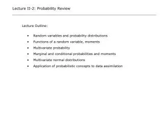
Lecture II-2: Probability Review. Lecture Outline: Random variables and probability distributions Functions of a random variable, moments Multivariate probability Marginal and conditional probabilities and moments Multivariate normal distributions

E N D
Lecture II-2: Probability Review • Lecture Outline: • Random variables and probability distributions • Functions of a random variable, moments • Multivariate probability • Marginal and conditional probabilities and moments • Multivariate normal distributions • Application of probabilistic concepts to data assimilation
Random Variables and Probability Density Functions fy (y) fy (y) All values between 0 and 1 are equally likely Smallest values are most likely 0 y 0 1 y Uniform distribution (e.g. soil texture) Exponential distribution (e.g. event rainfall) fy (y) 0.3 Probability that y = 2 0.25 0.2 0.15 0.1 Only discrete values (integers) are possible y 0 1 2 3 4 Discrete distribution (e.g. number of severe storms) A random variable is a variable whose possible values are distributed throughout a specified range. The variable’s probability density function (PDF) describes how these values are distributed (i.e. it gives the probability that the variable value falls within a particular interval). Continuous PDFs A Discrete PDF
Interval Probabilities f y(y) 0.4 0.2 0 -4 -2 0 2 4 y1 y1 y2 y2 y y f y(y) 0.4 0.2 0 -4 -2 0 2 4 Probability that x falls in interval (x1, x2]: Continuous PDF: Discrete PDF: Probability that y takes on some value in the range (- , + ) is 1.0: That is, area under PDF must = 1
Example: Calculating Interval Probabilities from a Continuous PDF 0.12 0.1 0.08 0.06 0.04 0.02 0 0 20 40 60 80 Historical data indicate that average rainfall intensity y during a particular storm follows an exponential distribution: a=0.1 mm -1 y (mm) What is the probability that a given storm will produce greater than 10mm. of rainfall if a=0.1 mm-1?
Cumulative Distribution Functions Cumulative distribution function (CDF) of x (probability that x is less than ): Continuous PDF: F y () Area = F y( ) 1 0.5 0.4 y y 0 -4 -2 0 2 4 0.2 Discrete PDF: 0 -4 -2 0 2 4 1 0.4 f y(y) F y () 0.5 0.2 0 0 -4 -2 0 2 4 y -4 -2 0 2 4 f y(y) y Note that F y () 1.0 !
Constructing PDFs and CDFs From Data y 2 0 -2 -4 0 10 20 30 40 50 t y Sample CDF 10 5 y Histogram (Sample PDF) 0 -3 -2 -1 0 1 2 How are these 50 monthly streamflows distributed over range of observed values? 1 0.8 Rank data from smallest to largest value and divide into bins (sample PDF or histogram) or plot normalized rank (rank/50) vs. value (sample CDF) 0.6 0.4 0.2 0 -3 -2 -1 0 1 2 Sample CDF may be fit with a standard function (e.g. Gaussian) 2
Expectation of a Random Variable Continuous: Discrete: The expectation of a function z = g(y) of the random variable y is defined as: Expectation is a linear operator: Note that expectation of y is not a random variable but is a property of the PDF f y(y ).
Moments and Other Properties of Random Variables Central Moments of y: Variance: Prob(y > median) = Prob(y median) =0.5 Mode (peak) Standard deviation: Median 0.35 0.3 1 Standard deviation 0.25 0.2 0.15 y95 0.1 Prob(y>y95) =0.05 0.05 0 0 2 4 6 8 10 12 14 Mean Non-central Moments of y: Mean: Second moment: Integrals are replaced by sums when PDF is discrete
Expectation Example Mean: Standard deviation: Mean defines “center” of distribution The mean and variance of a random variable distributed uniformly between 0 and 1 are: Variance: Standard deviation
Multiple (Jointly Distributed) Random Variables • We frequently work with groups of related random variables. • Discrete example: y1 = number of storms in June (0, 1, or 2) • y2 = number of storms in July (0, 1, or 2) f y1 y2 ( 0, 2 ) Table of joint (multivariate) probabilities: Assemble multiple random variables in vectors: y = [y1, y2 , …, yn ] f y1 y2 ( y1 , y2 ) 0.4 0.3 0.2 Shorthand: f y (y) = f y1 y2... yn (y1 , y2 ,..., yn ) 0.1 0 y1 2 y2 2 1 1 0 0 Plot table as discrete joint PDF with two independent variables y1 and y2
Interval Probabilities for Multivariate Random Variables 60 50 40 30 20 y2 10 2 10 20 30 40 50 60 1 0 y1 0 1 2 In multivariate problems interval probabilities are replaced by the probability that the n random variables fall in a specified region (R) of the n-dimensionalspace with coordinates ( y1 , y2 , …, yn ) . Bivariate case -- Probability that the pair of variables ( y1 , y2 ) lies in a region R in they1 - y2 plane is: y2 Continuous PDF (contour plot): Region R Discrete PDF (discrete contour plot): y1 0.15 Region R
General Multivariate Moments The mean of a vector of n random variables y = [y1, y2 , …, yn ] is an n vector: Second non-central moment of a vectory is an n by n matrix, called the covariance matrix: The correlation coefficient between any two scalar random variables (e.g. two elements of the vector y) is: If Cyiyk = ik= 0 then yi and yi are uncorrelated.
Marginal and Conditional PDFs The marginal PDF of any one of a set of jointly distributed random variables is obtained by integrating joint density over all possible values of the other variables. In the bivariate case marginal density of y1 is: Continuous PDF : Discrete PDF: The conditional PDF of a random variable yi for a given value of some other random variable yk is defined as: The conditional density of yi given yk is a valid probability density function (e.g. the area under this function must = 1).
Discrete Marginal and Conditional Probability Example For the discrete example described earlier the marginal probabilities are obtained by summing over columns [ to get f y1 ( y 1 )]or rows [ to get f y2 ( y 2 )] : Marginal densities shown in color (last row and last column) The conditional density of y1(June storms)given that y2 = 1 (one storm in July) is obtained by dividing the entries in the y2 = 1 column by f y2 ( y2=1) = 0.3:
Conditional Moments Conditional moments are defined in the same way as regular moments, except that the unconditional density [e.g. f y1 ( y1 )] is replaced by the conditional density [e.g. f y1|y2 (y1 |y12=1)] in the appropriate definitions. For discrete example, unconditional mean and variance of y1 may be computed directly from f y1 ( y1) table: The conditional mean and variance of y1given that y2 = 1 may be computed directly from f y1|y2 (y1 |y12=1)] table: Note that the conditional variance (uncertainty) of y1 is smaller than the unconditional variance. This reflects the decrease in uncertainty we gain by knowing that y12=1.
Independent Random Variables Two random vectors y and z are independent if any of the following equivalent expressions holds: Independent variables are also uncorrelated, although the converse may not be true. In the discrete example described above, the two random variables y and y are not independent because: For example, for the combination (y1= 0, y2= 0)we have:
Functions of a Random Variable z = g(y) = e y Corresponding range of z values 0.8 8 Range of possible y values 0.4 0.6 6 0.3 4 0.4 0.2 2 0.2 0.1 0 0 0 -2 -1 0 1 2 -4 0 -2 1 0 2 3 2 4 4 f z(z) (lognormal) f y(y) (normal) z = g (y) f y(y) f z(z) A function z = g(y) of a random variable is also a random variable, with its own PDF f z(z). The basic concept also applies to multivariate problems, where y and z are random vectors and z = g (y)is a vector transformation.
Derived Distributions An important example for data assimilation purposes is the simple scalar linear transformation z = g() = a + , where is a random variable with PDF f () and a is a constant. Then g -1(z) = z - a and the PDF of the random variable z is: The PDF f z(z) of the random variable z = g(y) may be sometimes be derived in closed form from g(y) and f z(z). When this is not possible Monte Carlo (stochastic simulation) methods may be used. If y and z are scalars and z = g(y) has a unique solutiony = g -1(z) for all permissibley, then: where: If z = g(y) has multiple solutions the right-hand side term is replaced by a sum of terms evaluated at the different solutions. This result extends to vectors of random variables and a vector transformation z = g(y) if the derivative g’is replaced by the Jacobian of g(y).
Bayes Theorem The definition of the conditional PDF may be applied twice to obtain Bayes Theorem, which is very important in data assimilation. To illustrate, suppose that we seek the PDF of a state vector y given that a measurement vector has the value z. This conditional PDF may be computed as follows.: This expression is useful because it may be easier to determine f z|y( z|y) and then compute f y|z( y|z) from Bayes Theorem than to derive f y|z( y|z) directly. For example, suppose that: Then if y is given (not random)f z | y(z| y) = f (z - y). If the unconditional PDFs f () and f y(y) are specified they can be substituted into Bayes Theorem to give the desired PDF f y|z( y|z). The specified PDFs can be viewed as prior information about the uncertain measurement error and state.
Multivariate Normal (Gaussian) PDFs The only widely used continuous joint PDF is the multivariate normal (or Gaussian): Multivariate normal PDF of the n vector y = [y1, y2 , …, yn ] is completely determined by mean and covarianceC yy of y: Where | C yy | represents determinant of C yy and C yy-1 represents inverse of C yy . f y1 y2 ( y1 , y2 ) Bivariate normal PDF: . Mean of normal PDF is at peak value. Contours of equal PDF form ellipses. y1 y2
Important Properties of Multivariate Normal Random Variables The following properties of multivariate normal random variables are frequently used in data assimilation: • A linear combination z = a1 y1+a2 y2+ … an yn = a T y of jointly normal random variables y = [y1 , y2 , … , yn]Tis also a normal random variable. The mean and variance of z are: • If y and z are multivariate normal random vectors with a joint PDF fyz(y, z)the marginal PDFs fy (y) and fz(z) and the conditional PDFs f y| z(y| z)and f z| y(z| y) are also multivariate normal. • Linear combinations of independent random variables become normally distributed as the number of variables approaches infinity (this is the Central Limit Theorem) • In practice, many other functions of multiple independent random variables also have nearly normal PDFs, even when the number of variables is relatively small (e.g. 10-100). For this reason environmental variables are often observed to be normally distributed.
Conditional Multivariate Normal PDFs and Moments (Conditional mean) (Conditional covariance) (y, z cross-covariance) (Normalization constant) • Consider two vectors of random variables which are all jointly normal: • y = [y1, y2 , …, yn ] (e.g. a vector of n states) • z = [z1, z2 , …, zm ] (e.g. a vector of m measurements) The conditional PDF of ygivenz is: Where: The conditional covariance is “smaller” than the unconditional y covariance (since the difference matrix [Cy y - Cyy| z] is positive definite). This decrease in uncertainty about y reflects the additional information provided by z
Application of Probabilistic Concepts to Data Assimilation • Data assimilation seeks to characterize the true but unknown state of an environmental system. Physically-based models help to define a reasonable range of possible states but uncertainties remain because the model structure may be incorrect and the model’s inputs may be imperfect. These uncertainties can be accounted for in an approximate way if we assume that the models inputs and states are random vectors. • Suppose we use a model and a postulated unconditional PDFf u ( u) for the input u to derive an unconditional PDFf y ( y) for the state y . f y ( y) characterizes our knowledge of the state before we include any measurements. • Now suppose that we want to include information contained in the measurement vector z . This measurement is also a random vector because it depends on the random state yand the random measurement error . The measurement PDF is f z ( z). • Our knowledge of the state after we include measurements is characterized by the conditional PDF f y|z (y| z). This density can be derived from Bayes Theorem. When y and z are multivariate normal f y|z (y| z) can be readily obtained from the multivariate normal expressions presented earlier. In other cases approximations must be made. • The estimates (or analyses) provided by most data assimilation methods are based in some way on the conditional density f y|z (y| z) .