Download

1 / 16
160 likes | 344 Views
Sanjiv Dinakar and Yözen Hernández. Genotyping of James Watson’s genome from Low-coverage Sequencing Data. Genetic Variation. Variations in the genome are called Single Nucleotide Polymorphisms ( SNPs ). Most of the genetic material between individuals is the same.

E N D
Sanjiv Dinakar and Yözen Hernández Genotyping of James Watson’s genomefrom Low-coverage Sequencing Data
Genetic Variation • Variations in the genome are called Single Nucleotide Polymorphisms (SNPs). • Most of the genetic material between individuals is the same. • SNPs make up < 1% of the human genome.
Genotypes • The possible values for a SNP are called alleles. • We consider only “bi-allelic” SNPs (SNPs with exactly two alleles in the human population). • Each person has two alleles for each SNP. • A “genotype” is said to be “homozygous” if the same allele is present in both copies and “heterozygous” if both alleles are present. A Heterozygous genotype
Shotgun Sequencing • “Shotgun sequencing” is the most popular method for sequencing genomes. • In shotgun sequencing, the DNA molecule is broken into many small, random fragments and the DNA sequence of each fragment is determined. These fragments are called “reads”. • The reference genome is then searched for each of these reads, to find the position in the genome, which the read most likely came from. • Since the position of SNPs within the reference genome is known, the alleles can be extracted from the reads.
James Watson's Genome • ~74.4 million reads from James Watson's genome are freely available on the internet (generated by Wheeler et al.) • These reads were generated using technology from 454 Life Sciences. • Wheeler used “DNA microarrays” from AffyMetrix, to genotype James Watson, but not all known SNPs were found. • Microarrays are expensive and can quickly become obsolete due to the reference genome changing. • We used different methods to determine the genotypes, based on the reads, and compared our results to those of Wheeler.
Our method • We need... • to have an already sequenced genome (reference genome) to compare this individual against. • to have a number of fragments derived from the individual's genome • to be able to locate where the fragments belong in the genome. • to know the location and alleles of the SNPs in the genome. • to determine whether both copies of the SNP are covered • The HapMap project stores a database of the alleles and position for most known SNPs. • The Human Genome Project, has created a reference genome, based on multiple volunteers. • If we're sure we've got both copies covered, then determining the genotype is easy.
Problems • The same copy may be sequenced much more often than the other or reads may be mapped to the wrong position in the genome. • Sequencing and mapping accuracy affect genotype determination. Using older methods, the genotype cannot be determined with a high confidence if the coverage is low. • It is estimated about 13x coverage is needed to accurate genotyping. • Can we determine genotypes with high accuracy from low-coverage data? How?
Read Mapping • In order to map the reads to the reference genome, Nucmer was used. • Nucmer uses the following procedure to map a read to the genome: • Find MUMs between the read and the reference genome, using suffix trees. • Cluster matches into closely grouped sets, dropping inconsistent matches. • Align the region between MUMs in each cluster.
Read mapping • After using Nucmer to map all the reads, we filtered Nucmer's output. • We removed: • all reads which were mapped to more than one position in the genome. • all reads which had more than 10 errors (substitutions, insertions, deletions) and less than 90% of the read covered by a cluster. • Using simulated reads (reads generated randomly from the reference genome, using ReadSim), this method achieved a 0.37% false positive rate. • Our accuracy was further improved by removing reads which gave an invalid allele.
SNP Genotyping • Once we have mapped the reads, we know what SNPs each read contains, but how do we find a SNP's genotype? • Binomial distribution: there are only two alleles per SNP, so the allele combinations for a heterozygous SNP follow a binomial distribution. • Using a binomial distribution, we can infer possible genotypes.
Locating and identifying SNPs • There is a tremendous number of SNPs to search through and this search needs to be done for each read. • A binary search algorithm is used to find the first SNP within the read. We want to find the SNP contained in the read with the smallest position. • Consecutive SNPs which follow the first SNP are included if they are contained in the read. • The base found at the SNP position is extracted, and counted if it is a valid allele. Otherwise, we assume there was an error in the read and the entire read is thrown out (because it indicates a possibly mismapped read). • Every time an allele is found, we update the heterozygous and corresponding heterozygous genotype probabilities, and move on to the next SNP.
Short Binary search example Read start:15928924 Read end: 15929185 List of SNPs ... ... 14431347 16010486 15700361 Look in the upper half... 15700375 16010486 15928971 This is it! Look at consecutive SNPs to see if any more are in the read...
“Calling” Genotypes • There may be many reads which contain the same SNP. We count the number of times an allele appears, and use known frequencies to calculate the genotype probability. • After all the reads have been processed, we can calculate the posterior probabilities using Bayes' Theorem: P(G|R)=P(G)*P(R|G)/P(R) Where P( G ) is given by Hardy-Weinberg proportions for known population allele frequencies f0 and f1 (i.e., P( G = {0,0} ) = f02 and P( G = {0,1} ) = 2 * f0 *f1). P(R|G={0,1})=(1/2)^|R| P(R|G={0,0})=P(error)^|R(1)|*(1-P(error))^|R(0)| P(R|G={1,1})=P(error)^|R(0)|*(1-P(error))^|R(1)| P(R)= P(R|G={0,1})*P( G={0,1} )+ P(R|G={0,0})*P( G={0,0} )+ P(R|G={1,1})*P( G={1,1})
Example • A SNP is overlapped with six reads. Four of the reads have the 0 allele, two of the reads have the 1 allele. • In the population, the 0 allele occurs 75% of the time, the 1 allele occurs 25% of the time. • Assume errors occur uniformly with a rate of 1% |R|=6, |R(1)|=2, |R(0)|=4 P( G = {0,1} )=2*0.75*0.25=0.375 P( G = {0,0} )=0.75*0.75=0.5625 P( G = {1,1} )=0.25*0.25=0.0625 P(R|G = {0,1} )=0.5^6=0.015625 P(R|G = {0,0} )=0.01^2*0.99^4=0.00009605 P(R|G = {1,1} )=0.01^4*0.99^2=0.000000009801 P(R)=0.015625*0.375+0.000096059601*0.5625+0.000000009801*0.0625=0.005913 P(G = {0,1}|R)=0.375*0.015625/0.005913=0.9909 P(G = {0,0}|R)=0.5625*0.00009605/0.005913=0.009137 P(G = {1,1}|R)=0.0625*0.000000009801/0.005913=.0000001036
Results • We compared our results with those of the team which sequenced Watson's genome. • Our binomial distribution calculations gave better results, calling more SNPs and giving better accuracy than Wheeler et al. did. • There are probabilistic models which are far superior to the simple binomial distribution, and which are more realistic biologically. We are currently working on implementing Hidden Markov Models to solve this problem.