Download
1 / 17
180 likes | 202 Views
Explore various methods and considerations for solving the Poloidal Field Diffusion Equation in fusion codes such as ASTRA and TRANSP. Discuss initial conditions, boundary conditions, and different strategies for current density evolution.

E N D
Options for Poloidal Field Diffusion Equation (PFDE) in ASTRA and TRANSP I. Voitsekhovitch. G. Pereverzev ISM/ITM meeting, Lisbon, 2010 Source of information: G. V. Pereverzev, P. N. Yushmanov IPP Report 5/98 2002 http://users.jet.efda.org/pages/t-task-force/Astra.pdf TRANSP manual: http://users.jet.efda.org/expert/transp/Help/HelpFile/transp_help_frame.htm
Motivation for this talk: D. Kalupin, ETS Code camp, July 2010, Cadarache initial q profile taken from one code may be inconsistent with total plasma current and equilibrium of another code ETS what modification of the initial q-profile should be allowed in ETS to solve this inconsistency? how this problem is solved in other codes?
Options for current density evolution: • solve PFDE (ASTRA, JETTO, TRANSP) • (2) Prescribed current density evolution: • 2a: prescribed current density (ASTRA) • 2b: prescribed q (ASTRA, TRANSP) • 2c: evolve the q profile using input Bp/Bt vs (R,t) or vs (R,t) where tan()=Bp/Bt (TRANSP) initial & bndry conditions consistency with: equilibrium? total plasma current? measured loop voltage? • TRANSP: • - time switching amongst the options (1) - (2b) and (2c) during run • in options (2b) and (2c), the solution of PFDE yields the resistivity profile (output)
Initial condition: practically not used Measured variables are but they involve 1st or 2nd derivative of () and equilibrium (V’, G2) Two types of initial conditions: j//(,t=0) = j0() Prescribed j(r). Current density is re-normalised to be consistent with Ipl Prescribed q(r) j//() is given, E//() is calculated using resistivity model Ipl is matched by applying some adjustment procedure E//() is flat (SS), j//() is calculated using resistivity model Ipl is not matched
Boundary conditions: At =B free-bndry code Simplified boundary conditions: a) Prescribed total plasma current: (ASTRA, TRANSP) (ASTRA, TRANSP) Total current may be not equal to experimental value b) Prescribed loop voltage: c) External circuit equation: (ASTRA)
Initial q-profile and total plasma current are prescribed – adjustment procedure in ASTRA Ipl is matched by adjusting surface current density (one grid point) (3 moment equilibrium) JET 71827, JETTO run seq. 178 Current, MA q Current density, MA/m2
Initial q-profile and total plasma current are prescribed – adjustment procedure in TRANSP - user selects the adjustment region 1 1; - the entire q profile is used without modification at < 1 - q profile is modified in the region, 1 to force consistency with total plasma current. This is done by adjusting the voltage profile using its analytic form: V() = V1 + V22 + (1 - (>1.25))2 • is a free parameter, its value is determined by one additional constraint: • =0 - use parabolic voltage profile • 2. match "q" at a particular radius • 3. match li/2+beta input data V1+V2 is the surface voltage, resistivity is adjusted to match total plasma current Adjusted voltage for selected resistivity model
Illustration of TRANSP options for JET Hybrid Scenario 75225 • Initial q-profile in TRANSP is taken from EFIT. Total plasma current is prescribed • EFIT and TRANSP (VMEC6 = Variational Moments Equilibrium Code)equilibrium are different • Modification of q-profile at the periphery? • Effect of these modifications on q-profile evolution?
Scan in initial conditions with narrow adjustment region (1=1):prescribed Ipl, q(r) and smoothed NCLASS for resistivity, calculatedV (red)prescribed Ipl, q(r) and loop voltage, calculated resistivity (blue) Resistivity,Ohm cm Current density NCLASS q zoom x10-5 Ohm cm voltage
Effect of different initial voltage on q-profile evolution q(=0) q(=0.7) Time, s
Scan in the width of adjustment region (1=0.8-1):prescribed Ipl, q(r), smoothed NCLASS for resistivity and calculated voltage (red)prescribed Ipl, q(r), loop voltage and calculated resistivity (blue) 1= 1 (solid), 0.8 (dotted-dashed) 1= 1 (solid), 0.8 (dotted-dashed) Current density Current density q q voltage voltage Modification of q is very small
Strongly inconsistent initial condition – increased q with fixed plasma current. Case with prescribed Vloop and computed resistivity qref (black), 1.5*qref & 1=0.85 (red),1.5*qref & 1=0.5 (blue) q Current density Voltage
Strongly inconsistent initial condition – reduced q with fixed plasma current. Case with prescribed Vloop and computed resistivity qref (black), qref/1.5 & 1=0.85 (red),qref/1.5 & 1=0.5 (blue) q Current density Voltage
Effect of initial condition on q-evolution Case with increased q/different 1 (colour) and reference q (black) Case with reduced q/different 1 (colour) and reference q (black) q(=0) q(=0) q(=0.7) q(=0.7) Time, s Time, s
Discussion: • More accurate (still simplified and fast) equilibrium model? • q adjustments and smoothing procedures? • Time switch between interpretative (prescribed q or j//) and predictive (PFDE) modes would be useful
TRANSP: summary of the option with input q–profile (and dq/dt) Given the q profile, Ampere's Law can be used to get profiles of either toroidal current density Jt or the useful flux surface averaged dot product <J.B> rotB = 4j/c Then, by Faraday's law, dq/dt ==> d/d(voltage profile) and the measured surface voltage is taken as the boundary value Then the current density <J.B> and electric field <E.B> profiles are available. Driven currents are supplied from other physics models (beams, bootstrap, LH). Then, from Ohm's Law, resis*(<J.B>-<J.B>driven) = <E.B> ==> resis = <E.B>/(<J.B>-<J.B>driven) and so the results of this analysis is a resistivity profile inferred from the input data.