Download
1 / 95
1.03k likes | 1.3k Views
Understandable Statistics Seventh Edition By Brase and Brase Prepared by: Lynn Smith Gloucester County College. Chapter Three Averages and Variation. Measures of Central Tendency. Mode Median Mean. The Mode. the value or property that occurs most frequently in the data. Find the mode:.

E N D
Understandable StatisticsSeventh EditionBy Brase and BrasePrepared by: Lynn SmithGloucester County College Chapter Three Averages and Variation
Measures of Central Tendency • Mode • Median • Mean
The Mode the value or property that occurs most frequently in the data
Find the mode: 6, 7, 2, 3, 4, 6, 2, 6 The mode is 6.
Find the mode: 6, 7, 2, 3, 4, 5, 9, 8 There is no mode for this data.
The Median the central value of an ordered distribution
To find the median of raw data: • Order the data from smallest to largest. • For an odd number of data values, the median is the middle value. • For an even number of data values, the median is found by dividing the sum of the two middle values by two.
Find the median: Data: 5, 2, 7, 1, 4, 3, 2 Rearrange: 1, 2, 2, 3, 4, 5, 7 The median is 3.
Find the median: Data: 31, 57, 12, 22, 43, 50 Rearrange: 12, 22, 31, 43, 50, 57 The median is the average of the middle two values =
The Mean The mean of a collection of data is found by: • summing all the entries • dividing by the number of entries
Find the mean: 6, 7, 2, 3, 4, 5, 2, 8
Sigma Notation The symbol means “sum the following.” is the Greek letter (capital) sigma.
Sample mean “x bar” Population mean Greek letter (mu) Notations for mean
Find the measure of center • Find the mode: 2,3,4,1,2,3,4,5,2,5,5,8,9,9,10 • Find the median: 5,3,4,10,2,3,9,5,2,5,2,8,4,9,1 • Find the mean: • 10, 9, 2, 9, 3, 8, 4, 5, 1, 5, 2, 2, 3, 5, 4 The sum of the numbers : 72 divided by the count 15 is the mean = 4.8 The median (middle): 4 There are two modes: 2 and 5 (bimodal data) These lists are all the same! Which is the best measure of center to report????
Number of entries in a set of data • If the data represents a sample, the number of entries = n. • If the data represents an entire population, the number of entries = N.
Resistant Measure a measure that is not influenced by extremely high or low data values
Mean Median The mean is less resistant. It can be made arbitrarily large by increasing the size of one value. The median is more resistant. It will not be heavily influenced by large or small values. Which is less resistant?
Midrange a measure of center that is the midpoint of a set of data
36,20,18,60,17,15,20,32,25,30 Order the list from smallest to largest 15,17, 18, 20, 20, 25, 30, 32, 36,60 Midrange = Compute the midrange:
Trimmed Mean a measure of center that is more resistant than the mean but is still sensitive to specific data values
To calculate a (5 or 10%) trimmed mean • Order the data from smallest to largest. • Delete the bottom 5 or 10% of the data. • Delete the same percent from the top of the data. • Compute the mean of the remaining 80 or 90% of the data.
15, 17, 18, 20, 20, 25, 30, 32, 36, 60 Delete the top and bottom 10% ( one value for every 10 random variables) New data list: 17, 18, 20, 20, 25, 30, 32, 36 10% trimmed mean = Compute a 10% trimmed mean:
Trimmed Mean Guidelines For 5% trimmed mean: Data sets n=3-20 ; drop min and max Data sets n=21 – 40 ; drop lowest 2 and highest 2 values, etc. For 10% trimmed mean: Data sets n=11-20 ; drop lowest 2 and highest 2 values Data sets n=21 – 30 ; drop lowest 3 and highest 3 values, etc.
Weighted Mean another measure of center that is more resistant than the mean but is still sensitive to specific data frequencies OR Average calculated where some of the numbers are assigned more importance or weight
To calculate a weighted mean • Order the data from least frequent to most frequent. • Multiply each value by its frequency or percentage. • Add the products and divide by the total frequency or total percentage (100% or 1.00).
Using our syllabus grading system, you have a test average of 77, quiz avg. of 91, homework avg. of 85, and classwork avg. of 100. 45% x 77 25% x 91 20% x 85 10% x 100 Weighted average= Compute a weighted mean:
Compute the Weighted Average: • Midterm grade = 92 • Term Paper grade = 80 • Final exam grade = 88 • Midterm weight = 25% • Term paper weight = 25% • Final exam weight = 50%
Compute the Weighted Average: • x w xw • Midterm 92 .25 23 • Term Paper 80 .25 20 • Final exam 88 .5044 • 1.0087
Mean of Grouped Data (Frequency Table) • Make a frequency table • Compute the midpoint (x) for each class. • Count the number of entries in each class (f). • Sum the f values to find n, the total number of entries in the distribution. • Treat each entry of a class as if it falls at the class midpoint.
Calculation of the mean of grouped data x (mdpt) 32 37 42 47 xf 128 185 84 423 Ages: f 30 - 34 4 35 - 39 5 40 - 44 2 45 – 49 9 xf = 820 f = 20
When do I use that? • Use the mode or midrange when the data appears to be uniform or unimodal but not symmetric; especially when there are extreme values to the left and right in the graph • Use the median when the data appears to be skewed or bimodal and symmetric; especially when there are extreme values to the left or right in the graph • Use the mean when the data appears to be somewhat symmetrical and unimodal; especially when the graph has very few extreme values
Measures of Variation • Range • Interquartile Range • Standard Deviation (Variance)
The Range (measure of spread most closely associated with mode or midrange as the center) the difference between the largest and smallest values of a distribution
Find the range: 10, 13, 17, 17, 18 The range = largest minus smallest = 18 minus 10 = 8
Interquartile Range (IQR) (measure of spread most closely associated with median as the center) the difference between the “low middle” and “high middle” or the middle 50% of a distribution • Percentiles that divide the data into fourths • Q1 = 25th percentile • Q2 = the median • Q3 = 75th percentile
Quartiles • Percentiles that divide the data into fourths • Q1 = 25th percentile • Q2 = the median • Q3 = 75th percentile
Quartiles Median = Q2 Q1 Q3 Lowest value Highest value Inter-quartile range = IQR = Q3 — Q1
Find the quartiles: 12 15 16 16 17 18 22 22 23 24 25 30 32 33 33 34 41 45 51 The data has been ordered. The median is 24.
Find the quartiles: 12 15 16 16 17 18 22 22 23 24 25 30 32 33 33 34 41 45 51 For the data below the median, the median is 17.5 17.5 is the first quartile.
Find the quartiles: 12 15 16 16 17 18 22 22 23 24 25 30 32 33 33 34 41 45 51 For the data above the median, the median is 33. 33 is the third quartile.
Find the interquartile range: 12 15 16 16 17 18 22 22 23 24 25 30 32 33 33 34 41 45 51 IQR = Q3 – Q1 = 33 – 17.5 = 15.5
The standard deviation a measure of the average variation of the data entries from the mean
Standard deviation of a sample mean of the sample n = sample size
To calculate standard deviation of a sample • Calculate the mean of the sample. • Find the difference between each entry (x) and the mean. These differences will add up to zero. • Square the deviations from the mean. • Sum the squares of the deviations from the mean. • Divide the sum by (n 1) to get the variance. • Take the square root of the variance to get the standard deviation.
The Variance the square of the standard deviation