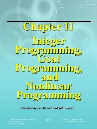
Integer Programming, Goal Programming, and Nonlinear Programming
Integer Programming, Goal Programming, and Nonlinear Programming. Chapter 11. To accompany Quantitative Analysis for Management , Tenth Edition , by Render, Stair, and Hanna Power Point slides created by Jeff Heyl. © 2009 Prentice-Hall, Inc. . Learning Objectives.


Integer Programming, Goal Programming, and Nonlinear Programming
E N D
Presentation Transcript
Integer Programming, Goal Programming, and Nonlinear Programming Chapter 11 To accompanyQuantitative Analysis for Management, Tenth Edition,by Render, Stair, and Hanna Power Point slides created by Jeff Heyl © 2009 Prentice-Hall, Inc.
Learning Objectives After completing this chapter, students will be able to: • Understand the difference between LP and integer programming • Understand and solve the three types of integer programming problems • Apply the branch and bound method to solve integer programming problems • Solve goal programming problems graphically and using a modified simplex technique • Formulate nonlinear programming problems and solve using Excel
Chapter Outline 11.1 Introduction 11.2 Integer Programming 11.3 Modeling with 0-1 (Binary) Variables 11.4 Goal Programming 11.5 Nonlinear Programming
Introduction • A large number of business problems can be solved only if variables have integer values • We will solve integer programming problems graphically and by using the branch and bound method • Many business problems have multiple objectives • Goal programming is an extension to LP that can permit multiple objectives • Linear programming requires linear models • Nonlinear programming allows objectives and constraints to be nonlinear
Integer Programming • An integer programming model is one where one or more of the decision variables has to take on an integer value in the final solution • There are three types of integer programming problems • Pure integer programming where all variables have integer values • Mixed-integer programming where some but not all of the variables will have integer values • Zero-one integer programming are special cases in which all the decision variables must have integer solution values of 0 or 1
Integer Programming • Solving an integer programming problem is much more difficult than solving an LP problem • Even the fastest computers can take an excessively long time to solve big integer programming problems • The most common technique used to solve integer programming problems is the branch and bound method
Harrison Electric Company Example of Integer Programming • The Company produces two products popular with home renovators, old-fashioned chandeliers and ceiling fans • Both the chandeliers and fans require a two-step production process involving wiring and assembly • It takes about 2 hours to wire each chandelier and 3 hours to wire a ceiling fan • Final assembly of the chandeliers and fans requires 6 and 5 hours respectively • The production capability is such that only 12 hours of wiring time and 30 hours of assembly time are available
Harrison Electric Company Example of Integer Programming • Each chandelier produced nets the firm $7 and each fan $6 • Harrison’s production mix decision can be formulated using LP as follows Maximize profit = $7X1 + $6X2 subject to 2X1 + 3X2 ≤ 12 (wiring hours) 6X1 + 5X2 ≤ 30 (assembly hours) X1, X2 ≥ 0 (nonnegative) where X1 = number of chandeliers produced X2 = number of ceiling fans produced
6 – 5 – 4 – 3 – 2 – 1 – 0 – X2 + + + + + + + + | | | | | | | 1 2 3 4 5 6 X1 Harrison Electric Company Example of Integer Programming • The Harrison Electric Problem 6X1 + 5X2 ≤ 30 + = Possible Integer Solution Optimal LP Solution (X1 =3.75, X2 = 1.5, Profit = $35.25) 2X1 + 3X2 ≤ 12 Figure 11.1
Harrison Electric Company Example of Integer Programming • The production planner Wes recognizes this is an integer problem • His first attempt at solving it is to round the values to X1 = 4 and X2 = 2 • However, this is not feasible • Rounding X2 down to 1 gives a feasible solution, but it may not be optimal • This could be solved using the enumeration method • Enumeration is generally not possible for large problems
Harrison Electric Company Example of Integer Programming • Integer solutions Optimal solution to integer programming problem Solution if rounding is used Table 11.1
Harrison Electric Company Example of Integer Programming • The rounding solution of X1 = 4, X2 = 1 gives a profit of $34 • The optimal solution of X1 = 5, X2 = 0 gives a profit of $35 • The optimal integer solution is less than the optimal LP solution • An integer solution can never be better than the LP solution and is usually a lesser solution
Branch-and-Bound Method • The most common algorithm for solving integer programming problems is the branch-and-bound method • It starts by first allowing non-integer solutions • If these values are integer valued, this must also be the solution to the integer problem • If these variables are not integer valued, the feasible region is divided by adding constraints restricting the value of one of the variables that was not integer valued • The divided feasible region results in subproblems that are then solved
Branch-and-Bound Method • Bounds on the value of the objective function are found and used to help determine which subproblems can be eliminated and when the optimal solution has been found • If a solution is not optimal, a new subproblem is selected and branching continues
Six Steps in Solving IP Maximization Problems by Branch and Bound • Solve the original problem using LP. If the answer satisfies the integer constraints, we are done. If not, this value provides an initial upper bound. • Find any feasible solution that meets the integer constraints for use as a lower bound. Usually, rounding down each variable will accomplish this. • Branch on one variable from step 1 that does not have an integer value. Split the problem into two subproblems based on integer values that are immediately above or below the noninteger value. • Create nodes at the top of these new branches by solving the new problem
Six Steps in Solving IP Maximization Problems by Branch and Bound 5. (a) If a branch yields a solution to the LP problem that is not feasible, terminate the branch (b) If a branch yields a solution to the LP problem that is feasible, but not an integer solution, go to step 6 (c) If the branch yields a feasible integer solution, examine the value of the objective function. If this value equals the upper bound, an optimal solution has been reached. If it not equal to the upper bound, but exceeds the lower bound, terminate this branch.
Six Steps in Solving IP Maximization Problems by Branch and Bound • Examine both branches again and set the upper bound equal to the maximum value of the objective function at all final nodes. If the upper bound equals the lower bound, stop. If not, go back to step 3. Note: Minimization problems involved reversing the roles of the upper and lower bounds
Harrison Electric Company Revisited • Recall that the Harrison Electric Company’s integer programming formulation is Maximize profit = $7X1 + $6X2 subject to 2X1 + 3X2 ≤ 12 6X1 + 5X2 ≤ 30 where X1 = number of chandeliers produced X2 = number of ceiling fans produced • And the optimal noninteger solution is X1 = 3.75 chandeliers, X2 = 1.5 ceiling fans profit = $35.25
Harrison Electric Company Revisited • Since X1 and X2 are not integers, this solution is not valid • The profit value of $35.25 will provide the initial upper bound • We can round down to X1 = 3, X2 = 1, profit = $27, which provides a feasible lower bound • The problem is now divided into two subproblems
Subproblem A Maximize profit = $7X1 + $6X2 subject to 2X1 + 3X2 ≤ 12 6X1 + 5X2 ≤ 30 X1≥ 4 Subproblem B Maximize profit = $7X1 + $6X2 subject to 2X1 + 3X2 ≤ 12 6X1 + 5X2 ≤ 30 X1≤ 3 Harrison Electric Company Revisited
Subproblem A’s optimal solution: [X1 = 4, X2 = 1.2, profit = $35.20] Subproblem B’s optimal solution: [X1 = 3, X2 = 2, profit = $33.00] Harrison Electric Company Revisited • If you solve both subproblems graphically • We have completed steps 1 to 4 of the branch and bound method
Next Branch (C) X1 = 4 X2 = 1.2 P = 35.20 X1≥ 4 Next Branch (D) X1 = 3.75 X2 = 1.5 P = 35.25 X1≤ 3 X1 = 3 X2 = 2 P = 33.00 Harrison Electric Company Revisited • Harrison Electric’s first branching: subproblems A and B Subproblem A Infeasible (Noninteger) Solution Upper Bound = $35.20 Lower Bound = $33.00 Upper Bound = $35.25 Lower Bound = $27.00 (From Rounding Down) Subproblem B Stop This Branch Solution Is Integer, Feasible Provides New Lower Bound of $33.00 Figure 11.2
Subproblem C Maximize profit = $7X1 + $6X2 subject to 2X1 + 3X2 ≤ 12 6X1 + 5X2 ≤ 30 X1≥ 4 X2 ≥ 2 Subproblem D Maximize profit = $7X1 + $6X2 subject to 2X1 + 3X2 ≤ 12 6X1 + 5X2 ≤ 30 X1≥ 4 X2 ≤ 1 Harrison Electric Company Revisited • Subproblem A has branched into two new subproblems, C and D
Harrison Electric Company Revisited • Subproblem C has no feasible solution because the all the constraints can not be satisfied • We terminate this branch and do not consider this solution • Subproblem D’s optimal solution is X1 = 4.17, X2 = 1, profit = $35.16 • This noninteger solution yields a new upper bound of $35.16
Subproblem E Maximize profit = $7X1 + $6X2 subject to 2X1 + 3X2 ≤ 12 6X1 + 5X2 ≤ 30 X1≥ 4 X1 ≤ 4 X2 ≤ 1 Subproblem D Maximize profit = $7X1 + $6X2 subject to 2X1 + 3X2 ≤ 12 6X1 + 5X2 ≤ 30 X1≥ 4 X1 ≥ 5 X2 ≤ 1 Harrison Electric Company Revisited • Finally we create subproblems E and F Optimal solution to E: X1 = 4, X2 = 1, profit = $34 Optimal solution to F: X1 = 5, X2 = 0, profit = $35
Harrison Electric Company Revisited • The stopping rule for the branching process is that we continue until the new upper bound is less than or equal to the lower bound • or no further branching is possible • The later case applies here since both branches yielded feasible integer solutions • The optimal solution is subproblem F’s node • Computer solutions work well on small and medium problems • For large problems the analyst may have to settle for a near-optimal solution
Subproblem C Subproblem A Subproblem D Subproblem F Subproblem E No Feasible Solution Region X1 = 4 X2 = 1.2 P = 35.20 X1 = 5 X2 = 0 P = 35.00 X1 = 4.17 X2 = 1 P = 35.16 X1 = 4 X2 = 1 P = 34.00 X2≥ 2 X1 = 3.75 X2 = 1.5 P = 35.25 X1≥ 4 X1≤ 4 X2≤ 1 Subproblem B X1 = 3 X2 = 2 P = 33.00 X1≤ 3 X1≥ 5 Upper Bound= $35.25 Lower Bound= $27.00 Harrison Electric Company Revisited • Harrison Electric’s full branch and bound solution Feasible, Integer Solution Optimal Solution Figure 11.3
Using Software to Solve Harrison Integer Programming Problem • QM for Windows input screen with Harrison Electric data Program 11.1A
Using Software to Solve Harrison Integer Programming Problem • QM for Windows solution screen for Harrison Electric data Program 11.1B
Using Software to Solve Harrison Integer Programming Problem • QM for Windows iteration results screen for Harrison Electric data Program 11.1C
Using Software to Solve Harrison Integer Programming Problem • Using Excel’s Solver to formulate Harrison’s integer programming model Program 11.2A
Using Software to Solve Harrison Integer Programming Problem • Integer variables are specified with a drop-down menu in Solver Program 11.2B
Using Software to Solve Harrison Integer Programming Problem • Excel solution to the Harrison Electric integer programming model Program 11.2C
Mixed-Integer Programming Problem Example • There are many situations in which some of the variables are restricted to be integers and some are not • Bagwell Chemical Company produces two industrial chemicals • Xyline must be produced in 50-pound bags • Hexall is sold by the pound and can be produced in any quantity • Both xyline and hexall are composed of three ingredients –A, B, and C • Bagwell sells xyline for $85 a bag and hexall for $1.50 per pound
Mixed-Integer Programming Problem Example • Bagwell wants to maximize profit • We let X = number of 50-pound bags of xyline • We let Y = number of pounds of hexall • This is a mixed-integer programming problem as Y is not required to be an integer
Mixed-Integer Programming Problem Example • The model is Maximize profit = $85X + $1.50Y subject to 30X + 0.5Y≤ 2,000 30X + 0.5Y≤ 800 30X + 0.5Y≤ 200 X, Y≤ 0 and X integer
Mixed-Integer Programming Problem Example • Using QM for Windows and Excel to solve Bagwell’s IP model Program 11.3
Mixed-Integer Programming Problem Example • Excel formulation of Bagwell’s IP problem with Solver Program 11.4A
Mixed-Integer Programming Problem Example • Excel solution to the Bagwell Chemical problem Program 11.4B
Modeling With 0-1 (Binary) Variables • We can demonstrate how 0-1 variables can be used to model several diverse situations • Typically a 0-1 variable is assigned a value of 0 if a certain condition is not met and a 1 if the condition is met • This is also called a binary variable
Capital Budgeting Example • A common capital budgeting problem is selecting from a set of possible projects when budget limitations make it impossible to select them all • A 0-1 variable is defined for each project • Quemo Chemical Company is considering three possible improvement projects for its plant • A new catalytic converter • A new software program for controlling operations • Expanding the storage warehouse • It can not do them all • They want to maximize net present value of projects undertaken
Capital Budgeting Example • Quemo Chemical Company information • The basic model is Maximize net present value of projects undertaken subject to Total funds used in year 1 ≤ $20,000 Total funds used in year 2 ≤ $16,000 Table 11.2
1 if catalytic converter project is funded 0 otherwise X1 = X2 = 1 if software project is funded 0 otherwise X3 = 1 if warehouse expansion project is funded 0 otherwise Capital Budgeting Example • The decision variables are • The mathematical statement of the integer programming problem becomes Maximize NPV = 25,000X1 + 18,000X2 + 32,000X3 subject to 8,000X1 + 6,000X2 + 12,000X3≤ 20,000 7,000X1 + 4,000X2 + 8,000X3≤ 16,000 X1, X2, X3= 0 or 1
Capital Budgeting Example • Solved with computer software, the optimal solution is X1 = 1, X2 = 0, and X3 = 1 with an objective function value of 57,000 • This means that Quemo Chemical should fund the catalytic converter and warehouse expansion projects only • The net present value of these investments will be $57,000
Limiting the Number of Alternatives Selected • One common use of 0-1 variables involves limiting the number of projects or items that are selected from a group • Suppose Quemo Chemical is required to select no more than two of the three projects regardless of the funds available • This would require adding a constraint X1 + X2 + X3≤ 2 • If they had to fund exactly two projects the constraint would be X1 + X2 + X3= 2
Dependent Selections • At times the selection of one project depends on the selection of another project • Suppose Quemo’s catalytic converter could only be purchased if the software was purchased • The following constrain would force this to occur X1 ≤ X2 or X1 – X2 ≤ 0 • If we wished for the catalytic converter and software projects to either both be selected or both not be selected, the constraint would be X1 = X2 or X1 – X2 = 0
Fixed-Charge Problem Example • Often businesses are faced with decisions involving a fixed charge that will affect the cost of future operations • Sitka Manufacturing is planning to build at least one new plant and three cities are being considered in • Baytown, Texas • Lake Charles, Louisiana • Mobile, Alabama • Once the plant or plants are built, the company want to have capacity to produce at least 38,000 units each year
Fixed-Charge Problem Example • Fixed and variable costs for Sitka Manufacturing Table 11.3
1 if factory is built in Baytown 0 otherwise X1 = 1 factory is built in Lake Charles 0 otherwise X2 = 1 if factory is built in Mobile 0 otherwise X3 = X4 = number of units produced at Baytown plant X5 = number of units produced at Lake Charles plant X6 = number of units produced at Mobile plant Fixed-Charge Problem Example • We can define the decision variables as
Minimize cost = 340,000X1 + 270,000X2 + 290,000X3 + 32X4 + 33X5 + 30X6 subject to X4 +X5 + X6≥ 38,000 X4≤ 21,000X1 X5≤ 20,000X2 X6≤ 19,000X3 X1,X2, X3 = 0 or 1; X4,X5, X6≥ 0 and integer • The optimal solution is X1 = 0,X2 = 1, X3 = 1, X4 = 0, X5 = 19,000, X6 = 19,000 Objective function value = $1,757,000 Fixed-Charge Problem Example • The integer programming formulation becomes