Download
1 / 27
270 likes | 431 Views
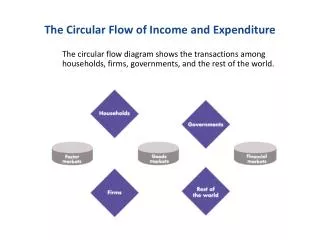
The circular flow of income and the Keynesian multiplier. Equilibrium in the goods market. Equilibrium in the goods market. The analysis of the goods market equilibrium is the starting point of Macroeconomic analysis (particularly from the Keynesian point of view)

E N D
The circular flow of income and the Keynesian multiplier Equilibrium in the goods market
Equilibrium in the goods market • The analysis of the goods market equilibrium is the starting point of Macroeconomic analysis (particularly from the Keynesian point of view) • All the goods and services are aggregated into a single market ⇒ 1 equation • The purpose is to find the equilibrium level of output Y* on this market ⇒ 1 unknown • A second issue is to describe how Y* varies as a function of other macroeconomic variables
Equilibrium in the goods market The circular flow of income Aggregate demand and output The multiplier and role of savings
Income € Labour Goods Expenditure€ The circular flow of income Households Firms
Labour Goods The circular flow of income Real flows Households Firms
Income € Expenditure€ The circular flow of income Monetary flows Households Firms
The circular flow of income • The circular flow of income is what guarantees the central accounting identities • Three definitions of GDP (output) • Sum of the expenditures Z • Sum of the value added produced Q • Sum of the incomes distributed Y • Accounting identities • Production = Aggregate demand / expenditure Q = Z • Production = Incomes of factors of production Q = Y
Equilibrium in the goods market The circular flow of income Aggregate demand and output The multiplier and role of savings
Aggregate demand and output • In the Keynesian model, the aggregate demand (also called planned expenditure) in a closed economy with no government is: Z = C + I with Z : Aggregate Demand C : Consumption of households I : Investment of firms
Aggregate demand and output • Consumption C is not fixed. Its level depends on the level of income Y, and is given by the consumption function. C = C0 + cY • Where • C0is the autonomous level of consumption, i.e. the level of consumption that does not depend on income • c is the marginal propensity to consume (mpc) : the amount spent out of an extra unit of income. • The converse is the marginal propensity to save (mps) s, such that c + s = 1
Aggregate demand and output • For the moment, investment I is considered to be exogenous. • Its level is pre-determined and does not depend on output • This is a simplifying assumption that will be relaxed later on (when interest rates are introduced) • Aggregate demand Z is therefore a function of output Y, of the marginal propensity to consume c and of the exogenous level of investment I. Z = C0 + cY + I
Aggregate demand and output Aggregate demand as a function of income Aggregate Demand Z Aggregate Demand (planned expenditure) Z = C0 + cY + I mpc: 0<c<1 Autonomous demand (not a function of Y) C0 + I Income, output Y
Aggregate demand and output • Effective demand and equilibrium • For any level of planned expenditure Z (with a slope < 1), There is only a single point for which the planned expenditure is equal to the level of income Y • This gives the equilibrium condition on the goods market: Y = Z • There is no guarantee that this point is a full employment equilibrium !! • This will be examined later.
Keynesian Equilibrium Output 45° Aggregate demand and output Equilibrium on the goods market Aggregate Demand Z Effective expenditure Y = Z Aggregate Demand (planned expenditure) Z = C0 + cY + I Income, output Y Y*
Aggregate demand and output • For each aggregate demand curve Z there is only a single point for which the planned expenditure is equal to the level of income Y • But Z is determined by the plans of agents! • What happens if the level of planned expenditure Z is not equal to Y ? • The goods market is not in equilibrium !! • Output will adjust so that the equilibrium is reached
Unplanned reduction in inventories The firms are selling more than they are producing. They have to increase production in order to meet the aggregate demand, which brings the goods market back to Y* Z Y 45° Aggregate demand and output Disequilibrium with Z > Y Aggregate Demand Z Effective expenditure Aggregate Demand (planned expenditure) Income, output Y Y Y*
Y Z Unplanned increase in inventories . Firms are selling less than they are producing. They reduce output which brings the goods market back to Y* 45° Aggregate demand and output Disequilibrium with Z < Y Aggregate Demand Z Effective expenditure Aggregate Demand (planned expenditure) Income, output Y Y Y*
Equilibrium in the goods market The circular flow of income Aggregate demand and output The multiplier and role of savings
The multiplier and the role of savings • So aggregate demand is given by Z = C + I • And the equilibrium condition is Y = Z • So what happens to output Y if investment I increases by an amount ΔI ? • In fact, ΔY > ΔI !! • Why is that?
45° The multiplier and the role of savings Multiplier effect on the goods market Aggregate Demand Z Y = Z Z2 = C0 + cY + I2 Z1 = C0 + cY + I1 1. An increase in planned investment… ΔI 2. …leads to a more than proportional increase in income ΔY Income, output Y Y1 Y2
The multiplier and the role of savings • Aggregate demand is given by : Z = C0 + cY + I • And Y = Z • Solving for the equilibrium level of output gives us : • There are 2 equivalent interpretations to this result Multiplier Autonomous demand (exogenous)
The multiplier and the role of savings Why do we observe ΔY > ΔI ? • First interpretation: a multiplier effect due to the circular flow of income Increase in savings ΔY × mps Increase in planned investment ΔI Increase in income ΔY Increase in consumption ΔY × mpc
The multiplier and the role of savings Why do we observe ΔY > ΔI ? • Step 1 : output increases by ΔI • Step 2 : output increases by c × ΔI • Step 3 : output increases by c2 × ΔI • Step 4 : output increases by c3 × ΔI • ..... This continues forever ! The closer c is to 1, i.e. the less people save, the larger the effect. (why ?) • The aggregate size of the increase is equal to:
The multiplier and the role of savings Why do we observe ΔY > ΔI ? • Second interpretation: The economy is increasing output in order to balance investments and savings • This is because the equilibrium condition Y=Z is equivalent to I=S (planned investment = savings) • These two equilibrium conditions are equivalent !
The multiplier and the role of savings • Aggregate demand can be decomposed into consumption and investment Z = C + I • Income can be decomposed into consumption and savings Y = Y(c+s) = C + S • So one can see that setting Y=Z is equivalent to setting I=S !
The multiplier and the role of savings Why do we observe ΔY > ΔI ? • Starting from equilibrium, if investment increases by ΔI, then we are no longer in equilibrium: • I + ΔI > S • To get back to equilibrium, we need savings to increase by the same amount (ΔS = ΔI). • Given the savings function, • So we have ⇒ ⇒
The multiplier and the role of savings Why do we observe ΔY > ΔI ? • Both explanations (spending multiplier or savings/investment balancing) are equally valid. • The spending multiplier is usually easier to understand, and is found in most manuals • The savings/investment balance, however, often brings more interesting explanations of the real-life economic phenomena.