Download
1 / 24
240 likes | 383 Views
Estimating the Likelihood of Statistical Models of Natural Image Patches. Daniel Zoran ICNC – The Hebrew University of Jerusalem Advisor: Yair Weiss. CifAR NCAP Summer School. Natural Image Statistics. Natural scenes and images exhibit very distinctive statistics

E N D
Estimating the Likelihood of Statistical Models of Natural Image Patches Daniel Zoran ICNC – The Hebrew University of Jerusalem Advisor: Yair Weiss CifAR NCAP Summer School
Natural Image Statistics • Natural scenes and images exhibit very distinctive statistics • A lot of research has been made in this field since the 1950s • Important in image processing, computer vision, computational neuroscience and more…
Natural Image Statistics Properties • The space of all possible images is huge • For a 256 gray levels, NxN sized matrix, there are possible images • Natural Images occupy a tiny fraction of this space • Some statistical properties of natural images: • Translation invariance • Power law spectrum – • Scale invariance • Non-Gaussianity of marginal statistics - (more on that later)
Estimating the Likelihood of different statistical models • During the years, a lot of models for natural image distributions have been proposed • It is hard to test the validity of such models, especially when comparing one model to the other • A step towards this – estimating the (log) likelihood of a given model and comparing the results with other models
Estimating the Likelihood of different models • Variable sized patches were extracted from natural images • Different models assumed • A training set was used to estimate various parameters of the model • Likelihood was calculated over a test set • 5000 patches in each set • Source images are mostly JPEGs from a Panasonic digital camera, portraying outdoor scenes • Also tested on standard images (Lena, Boat and Barbara – PNG format)
The models – 1D Gaussian • A 1D Gaussian distribution for every pixel • Mean and Variance estimated directly from the sample • The likelihood of an image x under this model is: • Where: • This model captures nothing about natural images
The models – Multidimensional Gaussian with PCA • Using the covariance matrix, rotate the images in the image space towards directions of maximum variance (PCA) • A Multidimensional Gaussian distribution for the components: • Where the covariance matrix is estimated from the training set: • This captures the Power-Law spectrum property
The models – Gaussian Mixture Model with PCA • Using the same rotation scheme (PCA), now assume a Gaussian Mixture Model for the marginal filter response distributions • Under this model: • Where W’s rows are the eigenvectors of the covariance matrix • The GMM parameters were found using EM • This captures both the Power-Law spectrum and the sparseness properties
The models – Generalized Gaussian with PCA • Finally, instead of using a GMM, we now use a Generalized Gaussian • This has the advantage of having less parameters, while still capturing Sparseness: • Parameters were obtained directly from the training set
The GG shape parameter • During the analysis of the data we have encountered a strange phenomena • Marginal distributions get wider as we go measure higher frequency filter responses • This is not due to increase in variance (which drops as we go to high frequencies) • We modeled this using the shape parameter obtained from the samples
Conclusion • This is (very) early work, still in progress • A lot of things left to do: • Try more models and filter (ICA is in progress) • Actually compare the different models • Try to make some sense out of the shape of the distributions • Look into higher order dependencies and correlations • A lot more…
Thank you! Questions?