Download
1 / 78
1.14k likes | 1.8k Views
ARCH/GARCH Models. Risk Management. Risk: the quantifiable likelihood of loss or less-than-expected returns. In recent decades the field of financial risk management has undergone explosive development.

E N D
Risk Management • Risk: the quantifiable likelihood of loss or less-than-expected returns. • In recent decades the field of financial risk management has undergone explosive development. • Risk management has been described as “one of the most important innovations of the 20th century”. • But risk management is not something new.
Risk Management José (Joseph) De La Vega was a Jewish merchant and poet residing in 17th century Amsterdam. There was a discussion between a lawyer, a trader and a philosopher in his book Confusion of Confusions. Their discussion contains what we now recognize as European options and a description of their use for risk management.
Risk Management • There are three major risk types: • market risk: the risk of a change in the value of a financial position due to changes in the value of the underlying assets. • credit risk: the risk of not receiving promised repayments on outstanding investments. • operational risk: the risk of losses resulting from inadequate or failed internal processes, people and systems, or from external events.
Risk Management • VaR (Value at Risk), introducedbyJPMorgan in the 1980s, is probably the most widely used risk measure in financial institutions.
Risk Management • Given some confidence level . The VaR of our portfolio at the confidence level α is given by the smallest value such that the probability that the loss exceeds is no larger than.
The steps to calculate VaR s t days to be forecasted market position Volatilitymeasure VAR Level of confidence Report of potential loss
The success of VaR Is a result of the method used to estimate the risk The certainty of the report depends upon the type of model used to compute thevolatilityonwhich these forecastisbased
Modeling Volatility withARCH & GARCH • In 1982,Robert Engle developed the autoregressive conditional heteroskedasticity (ARCH) models to model the time-varying volatility often observed in economical time series data. For this contribution, he won the 2003 Nobel Prize in Economics (*Clive Granger shared the prize for co-integration http://www.nobelprize.org/nobel_prizes/economic-sciences/laureates/2003/press.html). • ARCH models assume the variance of the current error term or innovation to be a function of the actual sizes of the previous time periods' error terms: often the variance is related to the squares of the previous innovations. • In 1986, his doctoral student Tim Bollerslev developed the generalized ARCH models abbreviated as GARCH.
Time series-ARCH (*Note, Zt can be other white noise, no need to be Gaussian) • Let be N(0,1). The process is an ARCH(q) process if it is stationary and if it satisfies, for all and some strictly positive-valued process, the equations • Where and , . • Note: is usually the error term in a time series regression model!
Time series-ARCH • ARCH(q) has some useful properties. For simplicity, we will show them in ARCH(1). • Without loss of generality, let a ARCH(1) process be represented by • Conditional Mean • Unconditional Mean • So have mean zero
Time series-ARCH • have unconditional variance given by • Proof 1 (use the law of total variance): Because it is stationary, . So .
Time series-ARCH • Proof 2: Lemma: Law of Iterated Expectations Let and be two sets of random variables such that . Let be a scalar random variable. Then Since, as ,
Time series-ARCH fatter tails • The unconditional distribution of Xt is leptokurtic, it is easy to show. • Proof: So.Also,
Time series-ARCH • The unconditional distribution of is leptokurtic, • The curvature is high in the middle of the distribution and tails are fatter than those of a normal distribution, which is frequently observed in financial markets.
Time series-ARCH • For ARCH(1), we can rewrite it as where • is finite, then it is an AR(1) process for . • Another perspective: • The above is simply the optimal forecast of if it follows an AR(1) process
Time series-EWMA • Before introducing GARCH, we discuss the EWMA (exponentially weighted moving average) model whereisa constant between 0 and 1. • The EWMA approach has the attractive feature that relatively little data need to be stored.
Time series-EWMA • We substitute for ,and then keep doing it for steps • For large , the term is sufficiently small to be ignored, so it decreases exponentially.
Time series-EWMA • The EWMA approach is designed to track changes in the volatility. • The value of governs how responsive the estimate of the daily volatility is to the most recent daily percentage change. • For example,the RiskMetricsdatabase, which was invented and then published by JPMorgan in 1994, uses the EWMA model with for updating daily volatility estimates.
Time series-GARCH • The GARCH processes are generalized ARCH processes in the sense that the squared volatility is allowed to depend on previous squared volatilities, as well as previous squared values of the process.
Time series-GARCH (*Note, Zt can be other white noise, no need to be Gaussian) • Let be N(0,1). The process is a GARCH(p, q) process if it is stationary and if it satisfies, for all and some strictly positive-valued process, the equations • Where and , , . • Note: is usually the error term in a time series regression model!
Time series-GARCH • GARCH models also have some important properties. Like ARCH, we show them in GARCH(1,1). • The GARCH(1, 1) process is a covariance-stationary white noise process if and only if . The variance of the covariance-stationary process is given by . • In GARCH(1,1), the distribution of is also mostly leptokurtic – but can be normal.
Time series-GARCH • We can rewrite the GARCH(1,1) as where • is finite, then it is an ARMA(1,1) process for Xt2.
Time series-GARCH • The equation for GARCH(1,1) can be rewritten as • where . • The EWMA model is a special case of GARCH(1,1) where
Time series-GARCH • The GARCH (1,1) model recognizes that over time the variance tends to get pulled back to a long-run average level of . • Assume we have known , if ,then this expectation is negative
Time series-GARCH • If ,then this expectation is positive • This is called mean reversion.
Time series-(ARMA-GARCH) • In the real world, the return processes maybe stationary, so we combine the ARMA model and the GARCH model, where we use ARMA to fit the mean and GARCH to fit the variance. • For example, ARMA(1,1)-GARCH(1,1)
Time Series in R Data from Starbucks Corporation (SBUX)
Program Preparation • Packages: >require(quantmod): specify, build, trade and analyze quantitative financial trading strategies >require(forecast): methods and tools for displaying and analyzing univariate time series forecasts >require(urca): unit root and cointegration tests encountered in applied econometric analysis are implemented >require(tseries): package for time series analysis and computational finance >require(fGarch): environment for teaching ‘Financial Engineering and Computational Finance’
Introduction >getSymbols('SBUX') >chartSeries(SBUX,subset='2009::2013')
Method of Modeling >ret=na.omit(diff(log(SBUX$SBUX.Close))) >plot(r, main='Time plot of the daily logged return of SBUX')
KPSS test • KPSS tests are used for testing a null hypothesis that an observable time series is stationary around a deterministic trend. • The series is expressed as the sum of deterministic trend, random walk, and stationary error, and the test is the Lagrange multiplier test of the hypothesis that the random walk has zero variance. • KPSS tests are intended to complement unit root tests
KPSS test where : contains deterministic components : stationary time series : pure random walk with innovation variance
Trend Check • KPSS test: null hypothesis: >summary(ur.kpss(r,type='mu',lags='short')) • Return is a stationary around a constant, has no linear trend
ADF test • ADF test is a test for a unit root in a time series sample. • ADF test: null hypothesis:has unit root • It is an augmented version of the Dickey-Fuller test for a larger and more complicated set of time series models. • ADF used in the test, is a negative number. The more negative it is, the stronger the rejection of the hypothesis that there is a unit root at some level of confidence.
Trend Check • ADF Test: null hypothesis: Xthas AR unit root (nonstationary) >summary(ur.df(r,type='trend',lags=20,selectlags='BIC')) • Return is a stationary time series with a drift
Check Seasonality • >par(mfrow=c(3,1)) >acf(r) >pacf(r) >spec.pgram(r)
Random Component • Demean data >r1=r-mean(r) >acf(r1); pacf(r1);
Random Component >fit=arima(r,order=c(1,0,0)) >tsdiag(fit) AR(1)
Random Component • First difference > diffr=na.omit(diff(r)) > plot(diffr); acf(diffr); pacf(diffr);
Random Component >fit1=arima(r,order=c(0,1,1)); tsdiag(fit1);
Random Component >fit2=arima(r,order=c(1,1,1)); tsdiag(fit2); ARIMA(1,1,1)
Model Selection where is the number of parameters, is likelihood Final model:
Shapiro-Wilk normality test • The Shapiro- Wilk test, proposed in 1965, calculates a W statistic that tests whether a random sample comes from a normal distribution. • Small values of W are evidence of departure from normality and percentage points for the W statistic, obtained via Monte Carlo simulations.