CHAPTER 3 Demand and Supply
1.32k likes | 2.37k Views
CHAPTER 3 Demand and Supply. Chapter 3 Demand, Supply and Relative Prices. Demand and supply determine relative prices. The word “price” means relative price. Price is an opportunity cost .

CHAPTER 3 Demand and Supply
E N D
Presentation Transcript
Chapter 3Demand, Supply and Relative Prices • Demand and supply determine relative prices. • The word “price” means relative price. Price is an opportunity cost. • If we predict a price will fall, we mean its price will fall relative to the average price of other goods and services.
Calculation of Relative Prices • Relative price is usually calculated by dividing the price of a good in question by a price index. • The most commonly used price index is the CPI (Consumer Price Index). • The CPI represents the “average” price of consumer goods in a particular month or year.
Demand • The quantity demanded of a good or service is the amount that consumers plan to (or are willing to) buy in a given period of time at a particular (relative) price. • Quantity demanded is measured as an amount per unit time: pizzas per day, pizzas per week, or pizzas per year.
The Law of Demand • Other things remaining the same, the higher the price of a good, the smaller is the quantity demanded. • The phrase “other things being equal” is sometimes abbreviated with the Latin phrase ceteris paribus(cet. par.). • Thus, when we say price changes, we mean relative price changes.
Demand Scheduleand Demand Curve • A demand schedule lists the quantities demanded at each different price when all the other influences on consumers’ planned purchases remain the same. • A demand curve is a graph of the demand schedule.
Demand Schedule a .50 9 b 1.00 6 c 1.50 4 d 2.00 3 e 2.50 2 Price Quantity Demanded (dollars per CD-R) (millions of CD-Rs per week)
Demand Curve 3.00 2.50 Price (dollar per CD-R) 2.00 1.50 1.00 .50 0 2 4 6 8 10 Quantity (millions of CD-Rs per week)
Demand Curve 3.00 e 2.50 Price (dollar per CD-R) d 2.00 c 1.50 b 1.00 a .50 0 2 4 6 8 10 Quantity (millions of CD-Rs per week)
Demand Curve 3.00 e 2.50 Price (dollar per CD-R) d 2.00 c 1.50 b 1.00 Demand for CD-Rs a .50 0 2 4 6 8 10 Quantity (millions of CD-Rs per week)
Factors ThatInfluence Demand • Price (of the good in question) • Prices of related goods • Income • Expected future price • Population • Preferences (or Tastes)
Price • If the price of the good rises, the quantitydemanded falls (a movement up along the demand curve). • If the price of the good falls, the quantitydemanded rises (a movement down along the demand curve).
Prices of Related Goods • A substitute is a good that can be used in place of another good. If the price of a CD-RW rises, the demand for CD-Rs rises (demand curve shifts out to the right) . • A complement is a good that is used in conjunction with another good. If the price of a CD burner rises, the demand for CD-Rs falls (demand curve shifts in to the left).
Example-Decrease in Price of a Complement Original demand schedule New demand schedule CD Burner $300 CD Burner $100 Price Quantity Price Quantity (dollars (millions of CD-Rs (dollars (millions of CD-Rs per CD-R) per week) per CD-R) per week)) a .50 9 b 1.00 6 c 1.50 4 d 2.00 3 e 2.50 2 Assume the original price of A CD Burner is $300. The demand schedule shows the Price-Quantity relationship for CD-Rs.
Example-Decrease in Price of a Complement Original demand schedule New demand schedule CD Burner $300 CD Burner $100 Price Quantity Price Quantity (dollars (millions of CD-Rs (dollars (millions of CD-Rs per CD-R) per week) per CD-R) per week)) a .50 9 a’ .50 13 b 1.00 6 b’ 1.00 10 c 1.50 4 c’ 1.50 8 d 2.00 3 d’ 2.00 7 e 2.50 2 e’ 2.50 6
Demand Before Price of Complement Decreases 3.00 2.50 e Price (dollar per CD-R) 2.00 d 1.50 c 1.00 b Demand for CD-Rs (CD Burner $300) .50 a 0 2 4 6 8 10 12 14 Quantity (millions of CD-Rs per week)
Demand after Price ofComplement Decreases 3.00 2.50 e e' Price (dollar per CD-R) Demand for CD-Rs (CD Burner $100) 2.00 d d' 1.50 c c' 1.00 b b' Demand for CD-Rs (CD Burner $300) .50 a a' 0 2 4 6 8 10 12 14 Quantity (millions of CD-Rs per week)
Income • Normal goods are those for which demand increases as income increases (demand curve shifts out to the right). • Inferior goods are those for which demand decreases as income increases (demand curve shifts in to the left). • The terms normal and inferior do not necessarily refer to the quality of the product
Expected Future Price • If the price of a good is expected to rise in the future and if the good can be stored, people will often substitute over time by buying more of the good today. • Demand for the good increases (demand curve shifts out to the right). This is sometimes called speculation.
Population • Other things remaining the same, the larger the population, the greater is the demand for all goods and services (demand curve shifts out to the right). • The smaller the population, the smaller is the demand for all goods and services (demand curve shifts in to the left).
Preferences (or Tastes) • Preferences are an individual’s attitudes toward goods and services. • Different people have different preferences and will therefore have different demands for a particular good or service.
Summary of Changes in Demand • Changes In Demand • The demand for CD-Rs • Decreases if: • The price of a substitute falls • The price of a complement rises • Income falls (since CD-R is a normal good) • The price of a CD-R is expected to fall in the future • The population decreases • Preferences decrease
Summary of Changes in Demand • Changes In Demand • The demand for CD-Rs • Increases if: • The price of a substitute rises • The price of a complement falls • Income rises (since CD-R is a normal good) • The price of a CD-R is expected to rise in the future • The population increases • Preferences increase
Movement Along Versus a Shift of the Demand Curve • If the price of a good changes but everything else remains the same, there is a movement along the demand curve. • If the price of a good remains constant but some other influence on buyers’ plans changes, there is a shift of the demand curve.
A Change in Quantity Demanded Versus a Change in Demand • A movement along the demand curve shows a change in the quantity demanded. • A shift of the demand curve shows a change in demand.
A Change in the Quantity Demanded Versus a Change in Demand Price D0 Quantity
A Change in the Quantity Demanded Versus a Change in Demand Price Decrease in quantity demanded Increase in quantity demanded D0 Quantity
A Change in the Quantity Demanded Versus a Change in Demand Price P0 D0 Quantity Q0
A Change in the Quantity Demanded Versus a Change in Demand Price P1 P0 D0 Quantity Q1 Q0
A Change in the Quantity Demanded Versus a Change in Demand Price P1 P0 P2 D0 Quantity Q1 Q0 Q2
A Change in the Quantity Demanded Versus a Change in Demand Price D0 Quantity
A Change in the Quantity Demanded Versus a Change in Demand Price Increase in demand D1 D0 Quantity
A Change in the Quantity Demanded Versus a Change in Demand Price Decrease in Increase in demand demand D1 D0 D2 Quantity
A Change in the Quantity Demanded Versus a Change in Demand Price Decrease in quantity demanded Decrease in Increase in demand demand Increase in quantity demanded D1 D0 D0 D2 Quantity
Supply • If a firm supplies a good or service, the firm • Has the resources and technology to produce it, • Can profit from producing it, and • Has made a definite plan to produce it and sell it.
Supply • The amount of a good or service that producers plan to (or are willing to) sell during a given time period at a particular price is called the quantity supplied. • Quantity supplied is not necessarily the same as the quantity actually sold (which depends on the interaction of supply and demand).
The Law of Supply • Other things remaining the same, the higher the price of a good, the greater is the quantity supplied. • Increasing opportunity cost is the reason behind the law of supply.
Supply Scheduleand Supply Curve • A supply schedule lists the quantities supplied at each different price when all other influences on the amount firms plan to sell remain the same. • A supply curve is a graph of a supply schedule.
Supply Schedule a .50 0 b 1.00 3 c 1.50 4 d 2.00 5 e 2.50 6 Price Quantity (dollars per CD-R) (millions of CD-Rs per week)
Supply Curve 3.00 2.50 Price (dollar per CD-R) 2.00 1.50 1.00 .50 0 2 4 6 8 10 Quantity (millions of CD-Rs per week)
Supply Curve 3.00 2.50 Price (dollar per CD-R) e 2.00 d 1.50 c 1.00 b .50 a 0 2 4 6 8 10 Quantity (millions of CD-Rs per week)
Supply Curve 3.00 Supply of CD-Rs 2.50 Price (dollar per CD-R) e 2.00 d 1.50 c 1.00 b .50 a 0 2 4 6 8 10 Quantity (millions of CD-Rs per week)
Other Influences on Supply Besides Price • Prices of factors of production • Prices of other goods produced • Expected future prices • The number of suppliers • Technology
Prices of Factorsof Production • A change in the price of a factor of production causes supply to change by changing production costs. • For example, suppose the product is automobiles and the price of labor increases. Automakers will cut back on their supply (the supply curve will shift to the left).
Prices of Related GoodsProduced - Substitutes • Two goods are substitutes in production if the same factors of production can be used to produce each good. Examples are sedans and sports cars. • If the price of sports cars rises, the quantity supplied of sports cars rises (move up the supply curve) and the supply of sedans falls (the supply curve of sedans shifts to the left).
Prices of Related GoodsProduced - Complements • Two goods are complements in production if they are produced together. Examples are beef and cowhide. • If the price of cowhide rises, the quantity supplied of cowhide rises (move up along the supply curve) and the supply of beef rises (the supply curve of beef shifts to the right).
Expected Future Prices • If producers expect the price of a good to be higher in the future (and the good can be stored), they may substitute over time. • This means they will offer a smaller quantity of the good for sale today so the current supply decreases (the supply curve shifts to the left) .
The Number of Suppliers • Other things remaining the same, the larger the number of producers supplying a good, the larger is the supply of the good (the supply curve shifts to the right).
Technology • New technologies that enable producers to use less (or cheaper) factors of production lower the cost of production and increase supply (the supply curve shifts to the right).
Supply Response to Change in Technology Original supply schedule Old technology Price Quantity (dollars (millions of CD-Rs per CD-R) per week) a .50 0 b 1.00 3 c 1.50 4 d 2.00 5 e 2.50 6