CS 326A: Motion Planning
340 likes | 358 Views
This motion planning approach uses trapezoidal decomposition to decompose the configuration space into "regular" regions and find targets in cluttered environments. It addresses issues such as property definition and decomposition usage. The approach is applicable in low-dimensional spaces but sensitive to floating point errors.

CS 326A: Motion Planning
E N D
Presentation Transcript
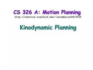
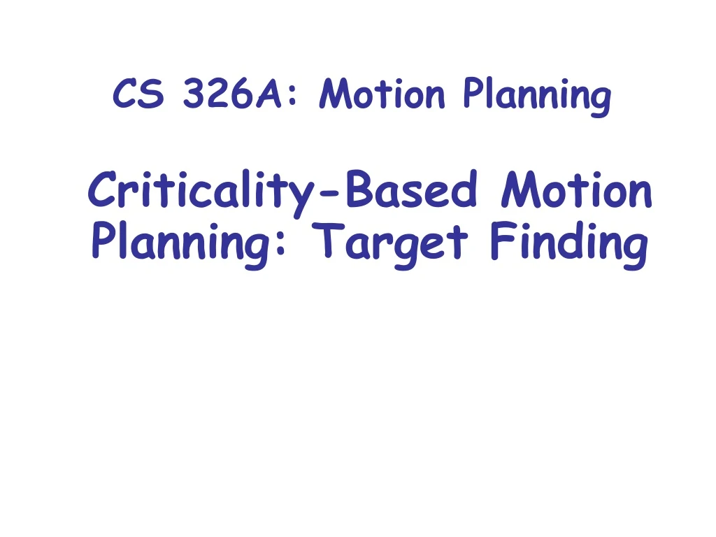
CS 326A: Motion Planning Criticality-Based Motion Planning: Target Finding
Criticality-Based Planning • Define a property P • Decompose the configuration space into “regular” regions (cells) over which P is constant. • Use this decomposition for planning • Issues: - What is P? It depends on the problem- How to use the decomposition? • Approach is practical only in low-dimensional spaces:- Complexity of the arrangement of cells- Sensitivity to floating point errors
Topics of this class and the next one • Target finding Information (or belief) state/space • Assembly planning Path space
cleared region 2 4 5 6 Example robot robot’s visibilityregion hiding region 1 3
Problem • A target is hiding in an environment cluttered with obstacles • A robot or multiple robots with vision sensor must find the target • Compute a motion strategy with minimal number of robot(s)
Assumptions • Target is unpredictable and can move arbitrarily fast • Environment is polygonal • Both the target and robots are modeled as points • A robot finds the target when the straight line joining them intersects no obstacles (omni-directional vision)
No ! Easy to test: “Hole” in the workspace Does a solution always existfor a single robot? Hard to test: No “hole” in the workspace
Two robots are needed Effect of Geometry on the Number of Robots
Effect of Number n of Edges Minimal number of robots N = Q(log n)
a = 0 or 1 c = 0 or 1 b = 0 or 1 (x,y) 0 cleared region 1 contaminated region Information State • Example of an information state = (x,y,a=1,b=1,c=0) • An initial state is of the form (x,y,a=1,b=1,...,u=1) • A goal state is any state of the form (x,y,a=0,b=0,..., u=0) visibility region free edge obstacle edge
b=1 b=0 a=0 a=0 cleared area b=1 a=0 Critical line Information state is unchanged (x,y,a=0,b=0) (x,y,a=0,b=1) Critical Line contaminated area (x,y,a=0,b=1)
Grid-Based Discretization • Ignores critical lines Visits many “equivalent” states • Many information states per grid point • Potentially very inefficient
Discretization into Conservative Cells In each conservative cell, the “topology” of the visibilityregion remains constant, i.e., the robot keeps seeing the same obstacle edges
Discretization into Conservative Cells In each conservative cell, the “topology” of the visibilityregion remains constant, i.e., the robot keeps seeing the same obstacle edges
Discretization into Conservative Cells In each conservative cell, the “topology” of the visibilityregion remains constant, i.e., the robot keeps seeing the same obstacle edges
Search Graph • {Nodes} = {Conservative Cells} X {Information States} • Node (c,i) is connected to (c’,i’) iff: • Cells c and c’ share an edge (i.e., are adjacent) • Moving from c, with state i, into c’ yields state i’ • Initial node (c,i) is such that: • c is the cell where the robot is initially located • i = (1, 1, …, 1) • Goal node is any node where the information state is (0, 0, …, 0) • Size is exponential in the number of edges
A (C,a=1,b=1) (B,b=1) (D,a=1) E B C D Example a b
A (C,a=1,b=1) (B,b=1) (D,a=1) E B C D (C,a=1,b=0) (E,a=1) Example
A (C,a=1,b=1) (B,b=1) (D,a=1) E B C D (C,a=1,b=0) (E,a=1) (B,b=0) (D,a=1) Example
A (C,a=1,b=1) (B,b=1) (D,a=1) E C D (C,a=1,b=0) (E,a=1) (B,b=0) (D,a=1) Example B Much smaller search tree than with grid-based discretization !
Visible Cleared Contaminated Example of Target-Finding Strategy
More Complex Example 2 1 3
Example with Recontaminations 3 1 2 6 4 5
Recontaminatedarea Example with Linear Number of Recontaminations 1 2 3 4
Example with Two Robots (Greedy algorithm)
Other Topics • Dimensioned targets and robots, three-dimensional environments • Non-guaranteed strategies • Concurrent model construction and target finding • Planning the escape strategy of the target