Section 8.2 Estimating When is Unknown
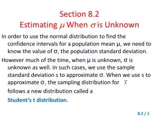
Section 8.2 Estimating When is Unknown. In order to use the normal distribution to find the confidence intervals for a population mean μ , we need to know the value of σ , the population standard deviation.

Section 8.2 Estimating When is Unknown
E N D
Presentation Transcript
Section 8.2Estimating When is Unknown In order to use the normal distribution to find the confidence intervals for a population mean μ, we need to know the value of σ, the population standard deviation. However much of the time, when μ is unknown, σ is unknown as well. In such cases, we use the sample standard deviation s to approximate σ. When we use s to approximate σ, the sampling distribution for follows a new distribution called a Student’s t distribution.
Student’s t Distributions The student’s t distribution uses a variable t defined as follows. A student’s t distribution depends on sample size n. Assume that x has a normal distribution with mean μ. For samples of size n with sample mean and standard deviation s, the t variable has a Student’s t distribution with degree of freedom d.f. = n – 1.
The shape of the t distribution depends only on the sample size, n, if the basic variable x has a normal distribution. When using the t distribution, we will assume that the x distribution is normal. Appendix Table 4 (Page A8)gives values of the variable t corresponding to the number of degrees of freedom (d.f.) d.f. = n – 1 where n = sample size
The t Distribution has a Shape Similar to that of the the Normal Distribution
Properties of a Student’s t Distribution 1. The distribution is Symmetric about the mean 0. 2. The distribution depends on the degrees of freedom (d.f. = b-1 for μ confidence intervals. 3. The distribution is Bell-shapedwith thicker tails than the standard normal distribution. 4. As the degrees of freedom increase, the t distribution approaches the standard normal distribution
Using Table 4 to find Critical Values for confidence Intervals Table 4 of the Appendix gives various t values for different degrees of freedom d.f. We will use the table to find the critical values for a c confidence level. In other words, we want to find such that the area equal to c under the t distribution for a given number of degrees of freedom falls between - and In the language of probability, we want to find such that This probability corresponds to the shaded area in next figure
Using Table 4 to Find Critical Values tc for a c Confidence Level
Using Table 4 to Find Critical Values of tc Find the column in the table with the given c heading Compute the number of degrees of freedom: d.f. = n 1 Read down the column under the appropriate c value until we reach the row headed by the appropriate d.f. If the required d.f. are not in the table: Use the closest d.f. that is smaller than the needed d.f. This results in a larger critical value tc. The resulting confidence interval will be longer and have a probability slightly higher than c.
Example: Find the critical value tc for a 95% confidence level for a t distribution with sample size n = 8. • Find the column in the table with c heading 0.950
Example cont. • Compute the number of degrees of freedom: • d.f. = n 1 = 8 1 = 7 • Read down the column under the appropriate c value until we reach the row headed by d.f. = 7
Example cont. tc = 2.365
PROCEDUREHow to find Confidence Intervals for When is Unknown c = confidence level (0 < c < 1) tc = critical value for confidence level c, and degrees of freedom d.f. = n 1
Example Confidence Intervals for , is Unknown The mean weight of eight fish caught in a local lake is 15.7 ounces with a standard deviation of 2.3 ounces. Construct a 90% confidence interval for the mean weight of the population of fish in the lake. Solution Mean = 15.7 ounces Standard deviation = 2.3 ounces. • n = 8, so d.f. = n – 1 = 7 • For c = 0.90, Appendix Table 4 gives t0.90 = 1.895.
Example cont. E= 1.54 The 90% confidence interval is: 15.7 - 1.54 < < 15.7 + 1.54 14.16 < < 17.24 We are 90% sure that the true mean weight of the fish in the lake is between 14.16 and 17.24 ounces.
Summary:Confidence intervals for the mean Assume that you have a random sample of size n > 1 from an x distribution and that you have computed and c. A confidence interval for μis Where E is the margin of error. How do you find E? It depends of how of how much you know about the x distribution.
Summary cont. Situation 1 (most common) You don’t know the population standard deviation σ. In this situation, you use the t distribution with margin of error and degree of freedom d.f. = n – 1 Although a t distribution can be used in many situations, you need to observe some guidelines. If n is less than 30, x should have a distribution that is mound-shaped and approximately symmetric. Its even better if the x distribution is normal. If n is 30 or more, the central limit theorem implies that these restrictions can be relaxed
Summary cont. Situation 2 (almost never happens!) You actually know the population value σ. In addition, you know that x has a normal distribution. If you don’t know that the x distribution is normal, then your sample size n must be 30 or larger. In this situation, you use the standard normal z distribution with margin of error
Summary cont. Which distribution should you use for Examine problem statement • If σis known use normal distribution with margin of error • If σis not known use Student’s t distribution with margin of error d.f. = n - 1 Assignment 20